Working with Sequences
CNTK Concepts
CNTK inputs, outputs and parameters are organized as tensors. Each tensor has a rank: A scalar is a tensor of rank 0, a vector is a tensor of rank 1, a matrix is a tensor of rank 2, and so on. We refer to these different dimensions as axes.
Every CNTK tensor has some static axes and some dynamic axes. The static axes have the same length throughout the life of the network. The dynamic axes are like static axes in that they define a meaningful grouping of the numbers contained in the tensor but:
- their length can vary from instance to instance
- their length is typically not known before each minibatch is presented
- they may be ordered
A minibatch is also a tensor. Therefore, it has a dynamic axis, called the batch axis, whose length can change from minibatch to minibatch. At the time of this writing CNTK supports a single additional dynamic axis. It is sometimes referred to as the sequence axis but it doesn’t have a dedicated name. This axis enables working with sequences in a high-level way. When operations on sequences are performed, CNTK does a simple type-checking to determine if combining two sequences is always safe.
To make this more concrete, let’s consider two examples. First, let’s see how a minibatch of short video clips is represented in CNTK. Suppose that the video clips are all 640x480 in resolution and they are shot in color which is typically encoded with three channels. This means that our minibatch has three static axes of length 640, 480, and 3 respectively. It also has two dynamic axes: the length of the video and the minibatch axis. So a minibatch of 16 videos each of which is 240 frames long would be represented as a 16 x 240 x 3 x 640 x 480 tensor.
Another example where dynamic axes provide an elegant solution is in learning to rank documents given a query. Typically, the training data in this scenario consist of a set of queries, with each query having a variable number of associated documents. Each of the query-document pairs includes a relevance judgment or label (e.g. whether the document is relevant for that query or not). Now depending on how we treat the words in each document we can either place them on a static axis or a dynamic axis. To place them on a static axis we can process each document as a (sparse) vector of size equal to the size of our vocabulary containing for each word (or short phrase) the number of times it appears in the document. However we can also process the document to be a sequence of words in which case we use another dynamic axis. In this case we have the following nesting:
- Query: CNTK
- Document 1:
- Microsoft
- Cognitive
- Toolkit
- Document 2:
- Cartoon
- Network
- Document 3:
- NVIDIA
- Microsoft
- Accelerate
- AI
- Query: flower
- Document 1:
- Flower
- Wikipedia
- Document 2:
- Local
- Florist
- Flower
- Delivery
The outermost level is the batch axis. The document level should have a dynamic axis because we have a variable number of candidate documents per query. The innermost level should also have a dynamic axis because each document has a variable number of words. The tensor describing this minibatch will also have one or more static axes, describing features such as the identity of the words in the query and the document. With rich enough training data it is possible to have another level of nesting, namely a session, in which multiple related queries belong to.
Sequence classification
One of the most exciting areas in deep learning is the powerful idea of recurrent neural networks (RNNs). RNNs are in some ways the Hidden Markov Models of the deep learning world. They are networks that process variable length sequences using a fixed set of parameters. Therefore they have to learn to summarize all the observations in the input sequence into a finite dimensional state, predict the next observation using that state and transform their current state and the observed input into their next state. In other words, they allow information to persist. So, while a traditional neural network layer can be thought of as having data flow through as in the figure on the left below, an RNN layer can be seen as the figure on the right.
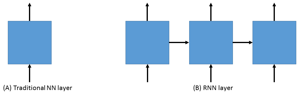
As is apparent from the figure above on the right, RNNs are the natural structure for dealing with sequences. This includes everything from text to music to video; anything where the current state is dependent on the previous state. While RNNs are indeed powerful, a “vanilla” RNN, whose state at each step is a nonlinear function of the previous state and the current observation, is extremely hard to learn via gradient based methods. Because the gradient needs to flow back through the network to learn, the contribution from an early element (for example a word at the start of a sentence) on much later elements, such as the classification of the last word in a long sentence, can essentially vanish.
Dealing with the above problem is an active area of research. An architecture that seems to be successful in practice is the Long Short Term Memory (LSTM) network. LSTMs are a type of RNN that are exceedingly useful and in practice are what we commonly use when implementing an RNN. A good explanation of the merits of LSTMs is at http://colah.github.io/posts/2015-08-Understanding-LSTMs. An LSTM is a differentiable function that takes an input and a state and produces an output and a new state.
In our example, we will be using an LSTM to do sequence classification. But for even better results, we will also introduce an additional concept here: word embeddings. In traditional NLP approaches, words are identified with the standard basis of a high dimensional space: The first word is (1, 0, 0, ...), the second one is (0, 1, 0, ...) and so on (also known as one-hot encoding). Each word is orthogonal to all others. But that is not a good abstraction. In real languages, some words are very similar (we call them synonyms) or they function in similar ways (e.g. Paris, Seattle, Tokyo). The key observation is that words that appear in similar contexts should be similar. We can let a neural network sort out these details by forcing each word to be represented by a short learned vector. Then in order for the network to do well on its task it has to learn to map the words to these vectors effectively. For example, the vector representing the word “cat” may somehow be close, in some sense, to the vector for “dog”. In our task we will learn these word embeddings from scratch. However, it is also possible to initialize with a pre-computed word embedding such as GloVe which has been trained on corpora containing billions of words.
Now that we’ve decided on our word representation and the type of recurrent neural network we want to use, let’s define the network that we’ll use to do sequence classification. We can think of the network as adding a series of layers:
- Embedding layer (individual words in each sequence become vectors)
- LSTM layer (allow each word to depend on previous words)
- Softmax layer (an additional set of parameters and output probabilities per class)
A very similar network is also located at Examples/SequenceClassification/SimpleExample/Python/SequenceClassification.py.
Let’s see how easy it is to work with sequences in CNTK:
import sys
import os
from cntk import Trainer, Axis
from cntk.io import MinibatchSource, CTFDeserializer, StreamDef, StreamDefs,\
        INFINITELY_REPEAT
from cntk.learners import sgd, learning_parameter_schedule_per_sample
from cntk import input_variable, cross_entropy_with_softmax, \
        classification_error, sequence
from cntk.logging import ProgressPrinter
from cntk.layers import Sequential, Embedding, Recurrence, LSTM, Dense

# Creates the reader
def create_reader(path, is_training, input_dim, label_dim):
    return MinibatchSource(CTFDeserializer(path, StreamDefs(
        features=StreamDef(field='x', shape=input_dim, is_sparse=True),
        labels=StreamDef(field='y', shape=label_dim, is_sparse=False)
        )), randomize=is_training,
        max_sweeps=INFINITELY_REPEAT if is_training else 1)


# Defines the LSTM model for classifying sequences
def LSTM_sequence_classifier_net(input, num_output_classes, embedding_dim,
                                LSTM_dim, cell_dim):
    lstm_classifier = Sequential([Embedding(embedding_dim),
                                  Recurrence(LSTM(LSTM_dim, cell_dim)),
                                  sequence.last,
                                  Dense(num_output_classes)])
    return lstm_classifier(input)


# Creates and trains a LSTM sequence classification model
def train_sequence_classifier():
    input_dim = 2000
    cell_dim = 25
    hidden_dim = 25
    embedding_dim = 50
    num_output_classes = 5

    # Input variables denoting the features and label data
    features = sequence.input_variable(shape=input_dim, is_sparse=True)
    label = input_variable(num_output_classes)

    # Instantiate the sequence classification model
    classifier_output = LSTM_sequence_classifier_net(
        features, num_output_classes, embedding_dim, hidden_dim, cell_dim)

    ce = cross_entropy_with_softmax(classifier_output, label)
    pe = classification_error(classifier_output, label)

    rel_path = ("../../../Tests/EndToEndTests/Text/" +
                "SequenceClassification/Data/Train.ctf")
    path = os.path.join(os.path.dirname(os.path.abspath(__file__)), rel_path)

    reader = create_reader(path, True, input_dim, num_output_classes)

    input_map = {
            features: reader.streams.features,
            label:    reader.streams.labels
    }

    lr_per_sample = learning_parameter_schedule_per_sample(0.0005)
    # Instantiate the trainer object to drive the model training
    progress_printer = ProgressPrinter(0)
    trainer = Trainer(classifier_output, (ce, pe),
                      sgd(classifier_output.parameters, lr=lr_per_sample),
                      progress_printer)

    # Get minibatches of sequences to train with and perform model training
    minibatch_size = 200

    for i in range(255):
        mb = reader.next_minibatch(minibatch_size, input_map=input_map)
        trainer.train_minibatch(mb)

    evaluation_average = float(trainer.previous_minibatch_evaluation_average)
    loss_average = float(trainer.previous_minibatch_loss_average)
    return evaluation_average, loss_average

if __name__ == '__main__':
    error, _ = train_sequence_classifier()
    print(" error: %f" % error)
Running this script should generate this output:
average      since    average      since      examples
   loss       last     metric       last
------------------------------------------------------
    1.61       1.61      0.886      0.886            44
    1.61        1.6      0.714      0.629           133
     1.6       1.59       0.56      0.448           316
    1.57       1.55      0.479       0.41           682
    1.53        1.5      0.464      0.449          1379
    1.46        1.4      0.453      0.441          2813
    1.37       1.28       0.45      0.447          5679
     1.3       1.23      0.448      0.447         11365
error: 0.333333
Let’s go through some of the intricacies of the network definition above. As usual, we first set the parameters of our model. In this case we
have a vocabulary (input dimension) of 2000, LSTM hidden and cell dimensions of 25, an embedding layer with dimension 50, and we have 5 possible
classes for our sequences. As before, we define two input variables: one for the features, and for the labels. We then instantiate our model. The
LSTM_sequence_classifier_net is a simple function which looks up our input in an embedding matrix and returns the embedded representation, puts
that input through an LSTM recurrent neural network layer, and returns a fixed-size output from the LSTM by selecting the last hidden state of the
LSTM:
lstm_classifier = Sequential([Embedding(embedding_dim),
                              Recurrence(LSTM(LSTM_dim, cell_dim))[0],
                              sequence.last,
                              Dense(num_output_classes)])
That is the entire network definition. In the second line above we select the first output from the LSTM. In this implementation of the LSTM this is the actual output while the second output is the state of the LSTM. We now simply set up our criterion nodes (such as how well we classify the labels using the thought vector) and our training loop. In the above example we use a minibatch size of 200 and use basic SGD with the default parameters and a small learning rate of 0.0005. This results in a powerful state-of-the-art model for sequence classification that can scale with huge amounts of training data. Note that as your training data size grows, you should give more capacity to the LSTM by increasing the number of hidden dimensions. Further, one can get an even more complex network by stacking layers of LSTMs. Conceptually, stacking LSTM layers is similar to stacking layers in a feedforward net. Selecting a good architecture however is very task-specific.
Feeding Sequences with NumPy
While CNTK has very efficient built-in readers that take care of many details for you (randomization, prefetching, reduced memory usage, etc.) sometimes your data is already in numpy arrays. Therefore it is important to know how to specify a sequence of inputs and how to specify a minibatch of sequences.
We have discussed text at length so far, so let’s switch gears and do an example with images. Feeding text data via NumPy arrays is not very different.
Each sequence must be its own NumPy array. Therefore if you have an input variable that represents a small color image like this:
x = sequence.input_variable((3,32,32))
and you want to feed a sequence of 4 images img1 to img4, to CNTK then you need to create a tensor containing all 4 images. For example:
img_seq = np.stack([img1, img2, img3, img4])
output = network.eval({x:[img_seq]})
The stack function in NumPy stacks the inputs along a new axis (placing it in the beginning by default) so the shape of img_seq is 4×3×32×32. You might have noticed that before binding img_seq to x we wrap it in a list. This list denotes a minibatch of 1 and minibatches are specified as lists. The reason for this is because different elements of the minibatch can have different lengths. If all the elements in the minibatch are sequences of the same length then it is acceptable to provide the minibatch as one big tensor of dimension b×s×d1×…×dk where b is the batch size, s is the sequence length and di is the dimension of the i-th static axis of the input variable.