Use CNTK learners

In CNTK, learners are implementations of gradient-based optimization algorithms. CNTK automatically computes the gradient of your criterion/loss with respect to each learnable parameter but how this gradient is combined with the current parameter value to provide a new parameter value is left to the learner.

CNTK provides three ways to define your learner, which we describe in detail in this notebook. You can - Use a built-in learner. Built-in learners are very fast. - Define your learner as a CNTK expression. This is not as fast as the built-in learners but more flexible. - Define your learner as a Python function. This is even more flexible but even less fast.

Here’s a “hello world” example for learners.

import cntk as C
import numpy as np
import math
np.set_printoptions(precision=4)

features = C.input_variable(3)
label = C.input_variable(2)
z = C.layers.Sequential([C.layers.Dense(4, activation=C.relu), C.layers.Dense(2)])(features)

sgd_learner_m = C.sgd(z.parameters, lr = 0.5, minibatch_size = C.learners.IGNORE)
sgd_learner_s2 = C.sgd(z.parameters, lr = 0.5, minibatch_size = 2)

We have created two learners here. sgd_learner_m is with a learning rate which is intended to be applied to any minibatches without considering their minibatich size; sgd_learner_s2 is with a learning rate which is intended to be applied to a minibatch of 2 samples.

When creating a learner we have to specify a learning rate schedule, which can be as simple as specifying a single number (0.5 in this example) or it can be a list of learning rates that specify what the learning rate should be at different points in time.

Currently, the best results with deep learning are obtained by having a small number of phases where inside each phase the learning rate is fixed and the learning rate decays by a constant factor when moving between phases. We will come back to this point later.

The minibatch_size parameter is the size of the minibatch that the learning rates are intended to apply to:

• minibatch_size = N: the learning rate is intended to be applied to N samples; if the actual minibatch size \(M\) is different from \(N\), CNTK scales the learning rate \(r\) by \(\frac{M}{N}\) so that the stepsize of the updates to the model parameters is the constant \(r\) for every \(N\) samples.
• minibatch_size = C.learners.IGNORE: the learning rate is applied the same way to minibatches of any size (ignoring the actual minibatch sizes).

Explanation with examples is given below.

To understand the difference and get familiar with the learner properties and methods, let’s write a small function that inspects the effect of a learner on the parameters assuming the parameters are all 0 and the gradients are all 1.

def inspect_update(learner, actual_minibatch_size, count=1):
    # Save current parameter values
    old_values = [p.value for p in learner.parameters]
    # Set current parameter values to all 0
    for p in learner.parameters:
        p.value = 0 * p.value
    # create all-ones gradients, and associate the sum of gradients over
    # the number of samples in the minibatch with the parameters
    gradients_sum = {p: np.zeros_like(p.value)
                     + 1.0 * actual_minibatch_size for p in learner.parameters}
    # do 'count' many updates
    for i in range(count):
        # note that CNTK learner's update function consumes
        # sum of gradients over the samples in a minibatch
        learner.update(gradients_sum, actual_minibatch_size)
    ret_values = [p.value for p in learner.parameters]
    # Restore values
    for p, o in zip(learner.parameters, old_values):
        p.value = o
    return ret_values

print('\nper minibatch:\n', inspect_update(sgd_learner_m, actual_minibatch_size=2))

per minibatch:
 [array([[-0.5, -0.5],
       [-0.5, -0.5],
       [-0.5, -0.5],
       [-0.5, -0.5]], dtype=float32), array([-0.5, -0.5], dtype=float32), array([[-0.5, -0.5, -0.5, -0.5],
       [-0.5, -0.5, -0.5, -0.5],
       [-0.5, -0.5, -0.5, -0.5]], dtype=float32), array([-0.5, -0.5, -0.5, -0.5], dtype=float32)]

With the knowledge that SGD is the update parameter = old_parameter - learning_rate * gradient, we can conclude that when the learning rate schedule is per minibatch, the learning rate \(0.5\) is applied to the mean gradient (which is \(1\) here by construction) of whole minibatch. Let’s see what happens when the learning rate schedule is per \(2\) samples.

print('\nper 2 samples: \n', inspect_update(sgd_learner_s2, actual_minibatch_size=2))

per 2 samples:
 [array([[-0.5, -0.5],
       [-0.5, -0.5],
       [-0.5, -0.5],
       [-0.5, -0.5]], dtype=float32), array([-0.5, -0.5], dtype=float32), array([[-0.5, -0.5, -0.5, -0.5],
       [-0.5, -0.5, -0.5, -0.5],
       [-0.5, -0.5, -0.5, -0.5]], dtype=float32), array([-0.5, -0.5, -0.5, -0.5], dtype=float32)]

We can conclude that when the learning rate schedule is per \(2\) samples, the learning rate \(0.5\) is also applied to the mean gradient of whole minibatch. Now let’s see what happens when the data minibatch size is set to \(10\) which is different from \(2\).

print('\nper minibatch:\n', inspect_update(sgd_learner_m, actual_minibatch_size=10))

per minibatch:
 [array([[-0.5, -0.5],
       [-0.5, -0.5],
       [-0.5, -0.5],
       [-0.5, -0.5]], dtype=float32), array([-0.5, -0.5], dtype=float32), array([[-0.5, -0.5, -0.5, -0.5],
       [-0.5, -0.5, -0.5, -0.5],
       [-0.5, -0.5, -0.5, -0.5]], dtype=float32), array([-0.5, -0.5, -0.5, -0.5], dtype=float32)]

Again we can conclude that when the learning rate schedule is per minibatch, the learning rate \(0.5\) is applied to the mean gradient of whole minibatch. Let’s see what happens when the learning rate schedule is per 2 samples.

print('\nper 2 samples: \n', inspect_update(sgd_learner_s2, actual_minibatch_size=10))

per 2 samples:
 [array([[-2.5, -2.5],
       [-2.5, -2.5],
       [-2.5, -2.5],
       [-2.5, -2.5]], dtype=float32), array([-2.5, -2.5], dtype=float32), array([[-2.5, -2.5, -2.5, -2.5],
       [-2.5, -2.5, -2.5, -2.5],
       [-2.5, -2.5, -2.5, -2.5]], dtype=float32), array([-2.5, -2.5, -2.5, -2.5], dtype=float32)]

We can see the interesting update pattern of how a per \(2\) sample learning rate \(0.5\) is applied. It updates the model with \(10 / 2 = 5\) times the mean gradient (which is \(1\)) with a learning rate \(0.5\) resulting in an update in the magnitute of \(5 \times 0.5 = 2.5\). Such a property is useful to update a model function whose loss function, when being evaluated at the current parameters, is locally linear within ball of a diameter of \(r \frac{M}{N}\) (where \(N\) is the specified minibatch size and \(M\) is the actual minibatch size). If we have an actual minibath size \(M > N\), this property allows us to increase the speed of updates aggressively; if \(M < N\), this property requires us to scale down the learning rate to increase the chance of convergence.

Please note that calling update manually on the learner (as inspect_update does) is very tedious and not recommended. Besides, you need to compute the gradients separately and pass them to the learner. Instead, using a **``Trainer``**, you don’t have to do any of that. The manual update used here is for educational purposes and for the vast majority of use cases CNTK users should avoid performing manual updates.

Trainers and Learners

A closely related class to the Learner is the Trainer. In CNTK, a Trainer brings together all the ingredients necessary for training models: - the model itself - the loss function (a differentiable function) and the actual metric we care about which is not necessarily differentiable (such as error rate) - the learners - optionally progress writers that log the training progress

While in the most typical case a Trainer has a single learner that handles all the parameters, it is possible to have multiple learners each working on a different subset of the parameters. Parameters that are not covered by any learner will not be updated. Here is an example that illustrates typical use.

sgd_learner = C.sgd(z.parameters, [0.05]*3 + [0.025]*2 + [0.0125], epoch_size=100)
loss = C.cross_entropy_with_softmax(z, label)
trainer = C.Trainer(z, loss, sgd_learner)
# use the trainer with a minibatch source as in the trainer howto

The trainer will compute the gradients of loss with respect to the parameters of z and call the sgd_learner’s update method as we did manually in the inspect_update function earlier. Here we have specified a learning rate schedule that is 0.05 for the first 300 minibatches (3 times the epoch size), then drops to 0.025 for the next 200 minibatches, and it is 0.0125 from then on until the end of training. This kind of functionality is quite common in tuning neural networks and it is the reason why in some papers (such as the ResNet paper) we see learning curves like this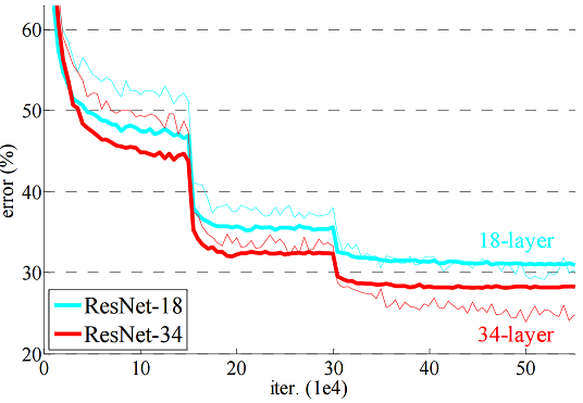

What is happening in this paper is that the learning rate gets reduced by a factor of 0.1 after 150000 and 300000 updates (cf. section 3.4 of the paper). In the example above the learning drops by a factor of 0.5 between each phase. Right now there is no good guidance on how to choose this factor, but it’s typically between 0.1 and 0.9.

Apart from specifying a Trainer yourself, it is also possible to use the cntk.Function.train convenience method. This allows you to specify the learner and the data and it internally creates a trainer that drives the training loop.

Other built-in learners

Apart from SGD, other built-in learners include - SGD with momentum (momentum_sgd) - SGD with Nesterov momentum (nesterov) first popularized in deep learning by this paper - Adagrad (adagrad) first popularized in deep learning by this paper - RMSProp (rmsprop) a correction to adagrad that prevents the learning rate from decaying too fast. - FSAdagrad (fsadagrad) adds momentum and bias correction to RMSprop - Adam / Adamax (adam(..., adamax=False/True)) see this paper - Adadelta (adadelta) see this paper

Momentum

Among these learners, FSAdaGrad, Adam, MomentumSGD, and Nesterov take an additional momentum schedule.

When using momentum, instead of updating the parameter using the current gradient, we update the parameter using all previous gradients exponentially decayed. If there is a consistent direction that the gradients are pointing to, the parameter updates will develop momentum in that direction. This page has a good explanation of momentum.

Like the learning rate schedule, the momentum schedule can be specified in two equivalent ways. Let use momentum_sgd as an example:

• momentum_sgd(parameters, momentum=float or list of floats, minibatch_size=C.leanrers.IGNORE, epoch_size=epoch_size)
  • or simply: momentum_sgd(parameters, momentum=float or list of floats, epoch_size=epoch_size) where minibatch_size=C.leanrers.IGNORE is the default
• momentum_sgd(parameters, momentum=float or list of floats, minibatch_size=minibatch_size, epoch_size=epoch_size)

As with learning_rate_schedule, the arguments are interpreted in the same way, i.e. there’s flexibility in specifying different momentum for the first few minibatches and for later minibatches:

• With minibatch_size=N, the decay momentum=\(\beta\) is applied to the mean gradient of every \(N\) samples. For example, minibatches of sizes \(N\), \(2N\), \(3N\) and \(k\cdot N\) will have decays of \(\beta\), \(\beta^2\), \(\beta^3\) and \(\beta^k\) respectively. The decay is exponetial in the proportion of the actual minibatch size to the specified minibath size.
• With minibatch_size=C.leanrers.IGNORE, the decay momentum=\(\beta\) is applied to the mean gradient of the whole minibatch regardless of its size. For example, regardless of the minibatch size being either \(N\) or \(2N\) (or any size), the mean gradient of such a minibatch will have same decay factor \(\beta\).

Apart from the momentum schedule, the momentum learners can also take a boolean “unit_gain” argument that determines the form of the momentum update:

• unit_gain=True: \(\textrm{momentum_direction} = \textrm{momentum} \cdot \textrm{old_momentum_direction} + (1 - \textrm{momentum}) \cdot \textrm{gradient}\)
• unit_gain=False: \(\textrm{momentum_direction} = \textrm{momentum} \cdot \textrm{old_momentum_direction} + \textrm{gradient}\)

The idea behind the non-conventional unit_gain=True is that when momentum and/or learning rate changes, this way of updating does not lead to divergence. In general, users should exercise great caution when switching learning rate and/or momentum with unit_gain=False. One piece of relevant advice is Remark 2 in this paper which shows how to adjust your momentum when the learning rate changes in the unit_gain=False case.

The following code illustrates that, for the case of unit_gain=False, the two ways of specifying momentum are equivalent. It also shows that when unit_gain=True you need to scale your learning rate by \(1/(1-\textrm{momentum})\) to match the unit_gain=False case

momentum = 0.9672161004820059
minibatch_size = 10
lr_schedule = C.learning_parameter_schedule(1, minibatch_size=C.learners.IGNORE)
ug_schedule = C.learning_parameter_schedule(1/(1-momentum), minibatch_size=C.learners.IGNORE)

m_schedule = C.momentum_schedule(momentum) #minibatch_size=C.learners.IGNORE
t_schedule = C.momentum_schedule(momentum, minibatch_size=minibatch_size)
#t_schedule is equivalent to the legacy API: (see the legacy interfaces section below for details)
#       t_schedule = C.momentum_as_time_constant_schedule(300)

msgd = C.momentum_sgd(z.parameters, lr_schedule, m_schedule, unit_gain=False)
tsgd = C.momentum_sgd(z.parameters, lr_schedule, t_schedule, unit_gain=False)
usgd = C.momentum_sgd(z.parameters, ug_schedule, m_schedule, unit_gain=True)

print(inspect_update(msgd, minibatch_size, 5)[0][0])
print(inspect_update(tsgd, minibatch_size, 5)[0][0])
print(inspect_update(usgd, minibatch_size, 5)[0][0])

[-14.3602 -14.3602]
[-14.3602 -14.3602]
[-14.3602 -14.3602]

Learners with individual learning rates

Among the built-in learners, adagrad, rmsprop, fsadagrad, adam, and adadelta have rules for tuning the learning rate of each parameter individually. They still require the tuning of a global learning rate that gets multiplied with the individual learning rate of each parameter. At the heart of these techniques is basically the idea that we can perform sgd on each parameter separately. This can be useful if some features appear less often than others and therefore different features are updated at different frequencies. With a single learning rate we run the risk of decaying it a lot before we see a rare feature (e.g. a rate word). Instead we might want the updates to depend on how often those features have been seen rather than how many minibatches have been processed.

These methods are typically easier to tune, but there is some new evidence that they overfit more easily than SGD with momentum.

Below, we show how these learners can be configured and how their updates affect the model parameters. The main take-away is that if you switch learners, you need to retune the learning rate. In this example the initial points and gradients are the same yet different learners arrive at different parameter values after 10 minibatches. Since the mean gradients are always 1, it is fair to say that in this case the learner with the most negative parameter value is the best. However, if we retune the learning rates, the learner with the least negative parameter value (fsadagrad, adam and adammax), we can drive its parameters to similar values as the ones with the very negative parameter value (e.g. adam, adamax and fsadagrad).

mb_size = 32

lr_schedule = C.learning_parameter_schedule(1, minibatch_size=C.learners.IGNORE)
t_schedule = C.momentum_schedule(0.971, minibatch_size=C.learners.IGNORE)

tsgd = C.momentum_sgd(z.parameters, lr_schedule, t_schedule, unit_gain=False)

adadelta  = C.adadelta(z.parameters, lr_schedule, 0.999, 1e-6)
adagrad   = C.adagrad(z.parameters, lr_schedule)
adam      = C.adam(z.parameters, lr_schedule, t_schedule, unit_gain=False)
adamax    = C.adam(z.parameters, lr_schedule, t_schedule, unit_gain=False, adamax=True)
fsadagrad = C.fsadagrad(z.parameters, lr_schedule, t_schedule, unit_gain=False)
rmsprop   = C.rmsprop(z.parameters, lr_schedule, gamma=0.999, inc=1.0+1e-9, dec=1.0-1e-9, max=np.inf, min=1e-30)

num_steps = 30
print('adadelta :', inspect_update(adadelta, mb_size, num_steps)[0][0])
print('adagrad  :', inspect_update(adagrad, mb_size, num_steps)[0][0])
print('adam     :', inspect_update(adam, mb_size, num_steps)[0][0])
print('adamax   :', inspect_update(adamax, mb_size, num_steps)[0][0])
print('fsadagrad:', inspect_update(fsadagrad, mb_size, num_steps)[0][0])
print('rmsprop  :', inspect_update(rmsprop, mb_size, num_steps)[0][0])

adadelta_schedule = C.learning_parameter_schedule(1004, minibatch_size=C.learners.IGNORE)
adadelta_tuned  = C.adadelta(z.parameters, adadelta_schedule, 0.999, 1e-6)
print('adadelta2:', inspect_update(adadelta_tuned, mb_size, num_steps)[0][0])

adadelta : [-0.0297 -0.0297]
adagrad  : [-30. -30.]
adam     : [-32.3197 -32.3197]
adamax   : [-32.3276 -32.3276]
fsadagrad: [-63.1707 -63.1707]
rmsprop  : [-30. -30.]
adadelta2: [-29.7969 -29.7969]

Writing a learner as a CNTK expression

If you want to experiment with your own learner, you should first try to write it as a CNTK expression. This is much faster than the next alternative, which is to write it in Python. CNTK has a universal learner that accepts a function as an argument. This function takes a list of parameters and gradients and creates an expression (a network) that, when evaluated, will assign new values to the parameters according to the learning rule you coded. At the time of this writing, the universal learner does not support schedules for learning rate and momentum. If this is necessary, the user must create a new learner. Another shortcoming of this learner is it only supports densely stored gradients. If you get an error that a quantity is not dense, you have two options: - Replace input variables that are sparse with dense (is_sparse=False) - Find the parameters with sparse gradients (typically those used at the very first layer) and use a built-in learner for those parameters

We are working to lift this requirement. Below we show how to write RMSprop using the universal learner.

def my_rmsprop(parameters, gradients):
    rho = 0.999
    lr = 0.01
    # We use the following accumulator to store the moving average of every squared gradient
    accumulators = [C.constant(1e-6, shape=p.shape, dtype=p.dtype) for p in parameters]
    update_funcs = []
    for p, g, a in zip(parameters, gradients, accumulators):
        # We declare that `a` will be replaced by an exponential moving average of squared gradients
        # The return value is the expression rho * a + (1-rho) * g * g
        accum_new = C.assign(a, rho * a + (1-rho) * g * g)
        # This is the rmsprop update.
        # We need to use accum_new to create a dependency on the assign statement above.
        # This way, when we run this network both assigns happen.
        update_funcs.append(C.assign(p, p - lr * g / C.sqrt(accum_new)))
    return C.combine(update_funcs)

my_learner = C.universal(my_rmsprop, z.parameters)
print(inspect_update(my_learner, 10, 2)[0][0])

[-0.5399 -0.5399]

Writing a learner as a Python class

CNTK expressions are very powerful and all the well-known learners can be expressed in this way. Still, there can be rare cases where you want to perform an update that cannot be currently implemented as a CNTK expression. In those cases you can implement your learner as a Python class. CNTK will then call its update method during training. Since this means the training loop (C++ code) is calling into Python (your learner) for every single minibatch, this approach is the slowest of all options.

In order for your class to be understood as a learner, it has to inherit from cntk.UserLearner. The constructor can be used to set up the learner. The trainer will call the learner’s update method by supplying it a dictionary, whose keys are the parameters and whose values are the corresponding gradients, as well as the number of samples in the minibatch and whether we have reached the end of a sweep through the data. The implementation of update is totally up to you.

In the code below, we create a learner that just performs SGD. In the constructor we create a dictionary mapping tensor shapes to CNTK expressions with the gradients being input variables. In the update method, for each parameter-gradient pair we look up the expression corresponding to the shape of the parameter, bind the gradient to the input of the expression and evaluate the expression. Finally, we slice the result to get rid of the batch axis and update the parameter. We have also slightly modified the inspect_update method to make it work with a user defined learner.

class MySgd(C.UserLearner):

    def __init__(self, parameters, lr_schedule):
        super(MySgd, self).__init__(parameters, lr_schedule, as_numpy=False)

        self.new_parameter = {}
        self.grad_input = {}

        self.sample_count_input = C.input_variable((), name='count')

        lr = lr_schedule[0]  # assuming constant learning rate
        eta = lr / self.sample_count_input

        # we need one graph per parameter shape
        for param in parameters:
            p_shape = param.shape
            self.grad_input[p_shape] = C.input_variable(p_shape)
            self.new_parameter[p_shape] = param - eta * self.grad_input[p_shape]

    def update(self, gradient_values, training_sample_count, sweep_end):
        for p, g in gradient_values.items():
            new_p = self.new_parameter[p.shape]
            grad_input = self.grad_input[p.shape]

            data = {
                    self.sample_count_input: np.asarray(training_sample_count),
                    grad_input: g
                    }
            result = new_p.eval(data, as_numpy=False)
            shape = result.shape

            # result has the shape of a complete minibatch, but contains
            # only one tensor, which we want to write to p. This means, we
            # have to slice off the leading dynamic axis.
            static_tensor = result.data.slice_view([0]*len(shape), shape[1:])
            p.set_value(static_tensor)
        return True

mb_size = 64
lr_schedule = C.learning_parameter_schedule(1, minibatch_size=C.learners.IGNORE)
my_sgd = MySgd(z.parameters, lr_schedule)

def inspect_user_learner_update(learner, mbsize, count):
    # user defined learner parameters are of type C.cntk_py.Parameter which is not nice to work with
    # we copy them out to easy_parameters and update their __class__ attribute to be C.Parameter
    easy_parameters = [p for p in learner.parameters()]
    for p in easy_parameters:
        p.__class__ = C.Parameter
    old_values = [p.value for p in easy_parameters]
    for p in easy_parameters:
        p.value = 0 * p.value
    updates = {p: p.value + 1 for p in easy_parameters}
    for i in range(count):
        learner.update(updates, np.float32(mbsize), sweep_end=False)
    ret_values = [p.value for p in easy_parameters]
    for p, o in zip(easy_parameters, old_values):
        p.value = o
    return ret_values

print(inspect_user_learner_update(my_sgd, mb_size, 10)[0][0])

[-0.1562 -0.1562]

And that’s all there is to learners! They are at the heart of neural network training, but by themselves they are not very useful, and they are typically driven by a trainer. So a good next step for you would be to take a look at our Trainer howto.

Legacy learner interfaces

Below, we explain how to use the learners with the legacy APIs prior to CNTK release 2.2. The APIs discussed below will be deprecated in future release. Please use the CNTK 2.2 or higher APIs explained above from now on.

Firstly, the learning rate schedule can be specified in two way in the legacy APIs:

lr_schedule_m = C.learning_rate_schedule(0.5, C.UnitType.minibatch)
lr_schedule_s = C.learning_rate_schedule(0.5, C.UnitType.sample)

sgd_learner_m = C.sgd(z.parameters, lr_schedule_m)
sgd_learner_s = C.sgd(z.parameters, lr_schedule_s)

We have created two learners here. When creating a learner we have to specify a learning rate schedule, which can be as simple as specifying a single number (0.5 in this example) or it can be a list of learning rates that specify what the learning rate should be at different points in time.

Currently, the best results with deep learning are obtained by having a small number of phases where inside each phase the learning rate is fixed and the learning rate decays by a constant factor when moving between phases. We will come back to this point later.

The second parameter in the learning rate schedule can be one of two different value: - Per minibatch - Per sample

To understand the difference and get familiar with the learner properties and methods, let’s inspect the effect of a learner on the parameters assuming the parameters are all 0 and the gradients are all 1.

print('\nunit = minibatch\n', inspect_update(sgd_learner_m, actual_minibatch_size=2))

unit = minibatch
 [array([[-0.5, -0.5],
       [-0.5, -0.5],
       [-0.5, -0.5],
       [-0.5, -0.5]], dtype=float32), array([-0.5, -0.5], dtype=float32), array([[-0.5, -0.5, -0.5, -0.5],
       [-0.5, -0.5, -0.5, -0.5],
       [-0.5, -0.5, -0.5, -0.5]], dtype=float32), array([-0.5, -0.5, -0.5, -0.5], dtype=float32)]

Recall that that SGD is the update parameter = old_parameter - learning_rate * gradient, we can conclude that when the learning rate schedule is per minibatch, the learning rate is aplied to the mean gradient of the whole minibatch. Let’s see what happens when the learning rate schedule is per sample.

print('\nunit = sample\n', inspect_update(sgd_learner_s, actual_minibatch_size=2))

unit = sample
 [array([[-1., -1.],
       [-1., -1.],
       [-1., -1.],
       [-1., -1.]], dtype=float32), array([-1., -1.], dtype=float32), array([[-1., -1., -1., -1.],
       [-1., -1., -1., -1.],
       [-1., -1., -1., -1.]], dtype=float32), array([-1., -1., -1., -1.], dtype=float32)]

In the per sample specification, the learning rate is applied to the gradient of individual sample instead of the mean gradient of the whole minibatch. CNTK offers both options because in some setups it is more convenient to work with per sample learning rates than per minibatch learning rates and vice versa.

Key concept: It is important to understand the ramifications of choosing learning rates per minibatch vs per sample. For example, per minibatch learning rate schedules, typically don’t require retuning when you want to change the minibatch size, but per sample schedules do. On the other hand with distributed training it is more accurate to specify the learning rate schedule as per sample rather than per minibatch.

Calling update manually on the learner (as inspect_update does) is very tedious and not recommended. Besides, you need to compute the gradients separately and pass them to the learner. Instead, using a Trainer, you don’t have to do any of that. The manual update used here is for educational purposes and for the vast majority of use cases CNTK users should avoid performing manual updates.

Momentum

Among these learners, momentum_sgd, nesterov, fsadagrad, and adam take an additional momentum schedule.

When using momentum, instead of updating the parameter using the current gradient, we update the parameter using all previous gradients exponentially decayed. If there is a consistent direction that the gradients are pointing to, the parameter updates will develop momentum in that direction. This page has a good explanation of momentum.

Like the learning rate schedule, the momentum schedule can be specified in two equivalent ways:

• momentum_schedule(float or list of floats, epoch_size)
• momentum_as_time_constant(float or list of floats, epoch_size)

As with learning_rate_schedule, the arguments are interpreted in the same way, i.e. there’s flexibility in specifying different momentum for the first few minibatches and for later minibatches.

The difference between the two calls is just a simple transformation as explained in the following. Since momentum is creating a sort of exponential moving average it is fair to ask “when does the contribution of an old gradient diminish by a certain constant factor?”. If we choose the constant factor to be \(0.5\) we call this the half-life and if we choose the constant to be \(e^{-1}\approx 0.368\) we call this the time constant. So momentum_as_time_constant_schedule specifies the number of samples it would take for the gradient of each minibatch to decay to \(0.368\) of its original contribution on the momentum term. Specifying a momentum_as_time_constant_schedule(300) and a minibatch size of 10 is a little bit more meaningful than specifying momentum_schedule(.967...) even though both lead to the same updates. The way to convert between the two schedules is - \(\textrm{momentum} = \exp(-\frac{\textrm{minibatch_size}}{\textrm{time_constant}})\) - \(\textrm{time_constant} = \frac{\textrm{minibatch_size}}{\log(1/\textrm{momentum})}\)

mb_size = 10
time_constant = 300
momentum = math.exp(-mb_size/time_constant)

print('time constant for momentum of 0.967... = ', mb_size/math.log(1/momentum))
print('momentum for time constant of 300      = ', math.exp(-mb_size/time_constant))

time constant for momentum of 0.967... =  300.00000000000006
momentum for time constant of 300      =  0.9672161004820059

Apart from the momentum schedule, the momentum learners can also take a boolean “unit_gain” argument that determines the form of the momentum update:

• unit_gain=True: \(\textrm{momentum_direction} = \textrm{momentum} \cdot \textrm{old_momentum_direction} + (1 - \textrm{momentum}) \cdot \textrm{gradient}\)
• unit_gain=False: \(\textrm{momentum_direction} = \textrm{momentum} \cdot \textrm{old_momentum_direction} + \textrm{gradient}\)

The idea behind the non-conventional unit_gain=True is that when momentum and/or learning rate changes, this way of updating does not lead to divergence. In general, users should exercise great caution when switching learning rate and/or momentum with unit_gain=False. One piece of relevant advice is Remark 2 in this paper which shows how to adjust your momentum when the learning rate changes in the unit_gain=False case.

The following code illustrates that, for the case of unit_gain=False, the two ways of specifying momentum (as time constant or not) are equivalent. It also shows that when unit_gain=True you need to scale your learning rate by \(1/(1-\textrm{momentum})\) to match the unit_gain=False case

lr_schedule = C.learning_rate_schedule(1, C.UnitType.minibatch)
ug_schedule = C.learning_rate_schedule(1/(1-momentum), C.UnitType.minibatch)

m_schedule = C.momentum_schedule(momentum)
t_schedule = C.momentum_as_time_constant_schedule(time_constant)

msgd = C.momentum_sgd(z.parameters, lr_schedule, m_schedule, unit_gain=False)
tsgd = C.momentum_sgd(z.parameters, lr_schedule, t_schedule, unit_gain=False)
usgd = C.momentum_sgd(z.parameters, ug_schedule, m_schedule, unit_gain=True)

print(inspect_update(msgd, mb_size, 5)[0][0])
print(inspect_update(tsgd, mb_size, 5)[0][0])
print(inspect_update(usgd, mb_size, 5)[0][0])

[-14.3602 -14.3602]
[-14.3602 -14.3602]
[-14.3602 -14.3602]