from IPython.display import Image

Network Optimizations

In recent years, the DNN Research community has proposed many techniques to make inference faster and more compact. Proposed techniques include factoring matrix-vector-product and convolution operations, binarization/quantization, sparsification and the use of frequency-domain representations.

The goal of cntk.contrib.netopt module is to provide users of CNTK easy-to-use interfaces to speed up or compress their networks using such optimizations, and writers of optimizations a framework within which to export them to CNTK users. The initial release of netopt supports factoring of Dense CNTK layers and the 1-bit binarization of Convolutional layers.

The manual shows how to use the netopt module to optimize CNTK networks.

Description

netopt breaks down the process of optimizing models into three steps:

1. Replace operations (or blocks) in the network with “cheaper”, possibly user-defined operations that are trainable, i.e., have forward and back-prop functions defined. We call the resulting network the transformed network.
2. [Optionally] Retrain the transformed network. Almost always, the transformation results in a significant drop in accuracy, and re-training the transformed version fairly quickly regains some/much of the lost accuracy.
3. [Optionally] Replace operations in the retrained network with operations that have fast implementations on particular processor architectures (e.g., they may require Intel AVX or ARM Neon acceleration). These new “lower-level” operations may not be trainable (i.e., have no back-prop functions defined), can only be run in forward mode, and are often user-defined. We call the resulting network a lowered network. Lowering is sometimes necessary to harvest the benefits of optimization. For example, a binarized convolution layer is only useful if the new layer is implemented using a lowered version of the convolution algorithm optimized for 1-bit values, as opposed to the standard convolution algorithmt that works on floats.

Each optimization provided via network should take as argument a model to be optimized, an optional training function for that model, and other optional arguments specific to that optimization, and return a model (possibly in a lowered representation) on which the above sequence of transformation, training and lowering has been performed.

Factorization of dense layers

This optimization, accessed via factorization.factor_dense(.) function, replaces Dense layers with factored variants. In particular, a dense layer encapsulates the operation r = W*x + b. If W is of shape m*n, this operation will take O(mn) operations. Now consider a (approximate) factorization of W: W ~ UV, where U has shape m*k and V has shape k*n. If we replace r with r’ = (U * (V*x)) + b, then computing r’ will take O(mk + kn) operations. If k is much smaller than m or n, this can yield large savings. netopt allows users to optionally specify a “factorization function” to use to derive U and V from W. Alternately, it allows users to specify a “rank function” that can examine W and derive a rank k that should be used for factorization. In this case, which we expect to the be common use case, netopt will perform a rank-k singular-value decomposition to produce U and V.

netopt.examples.dense_factorization_example() shows how to use dense factorization to transform a graph. In this example, no re-training of the transformed graph is performed. Further, factorization does not require lowering of the transformed graph, since the operations used by the transformed graph (matrix-vector multiply over floats) already has an efficient implementation in CNTK.

Using Factorization

We will use CNTK 102: Feed Forward Network with Simulated Data tutorial to demonstrate the use of factorization. We assume you have a working version of the code for the above tutorial and will show how to introduce factorization.

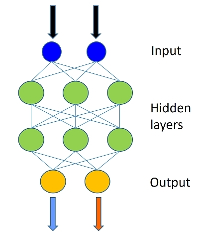
The feed forward network created for the above tutorial will be relatively simple with 2 hidden layers (num_hidden_layers) with each layer having 50 hidden nodes (hidden_layers_dim):

# Figure 1
Image(url="http://cntk.ai/jup/feedforward_network.jpg", width=200, height=200)

Once the training is completed, we have a model, denoted z, that can be optimized with factorization.

The two hidden (dense) layers in this network are fully connected and hence good candidates for the factorization optimization.

We will use the cntk.contrib.netopt.factorization.factor_dense function to factor these layers.

factor_dense has the signature:

factor_dense(model:Function,
             projection_function=None:np.ndarray->int
             filter_function=None:Function->bool
             factor_function=None:np.ndarray*int->(np.ndarray*np.ndarray))
-> Function

It takes as input a model and returns the transformed model. Futher: 1. filter_function selects which dense blocks (or layers) to factor. It is applied to every dense block, and the block is only transormed if filter_function returns true. 2. For every weight matrix W in a dense block, projection_function(W) returns the rank k that the factored matrices should have. 3. If factor_function is provided, then W will be factored into U, V = factor_function(W, k). If not, W will be factored into dot(U, dot(diag(S), V)) where U, S, V = np.linalg.svd(W)

We first consider an example where we transform every dense block (so the default filter_function remains) and we use a rank of each W is 60% of its smaller dimension. Further, we use the default SVD-based factoring, so that factor_function is unchanged.

# import netopt module
import cntk.contrib.netopt.factorization as nc

# example function determining the rank of the factorization.
def get_reduced_rank(W):
    # The rank of a matrix is at most the length of its smallest side.
    # We require the factored version to have a fraction of this original rank.
    return int(min(W.shape) * 0.6)

# newz will have all its Dense layers with their factored variants.
newz = nc.factor_dense(z, projection_function=get_reduced_rank)

Alternatively, consider the case where we wish to factor only the dense blocks that are square. In the current example, this will exclude the input dense layer. We can use the filter_function optional argument as follows:

# A function to select the layers to apply the optimization. Here we require that the layer
# has a square weight matrix, thus selecting for the second dense layer in our model.
def dense_filter(block):
    d1, d2 = block.W.value.shape
    return d1 == d2

# newz will have its second dense layer replaced with optimized dense layer.
newz = nc.factor_dense(z, projection_function=get_rank, filter_function=dense_filter)

Evaluating the factorized network

Once the optimization is completed, we can evaluate the new model using the same evaluation steps as the original network:

out = C.softmax(newz)

predicted_label_probs = out.eval({input : features}) #evaluate the new model
print("Label    :", [np.argmax(label) for label in labels]) #original labels
print("Predicted:", [np.argmax(row) for row in predicted_label_probs])

Binarization of convolution operations

This optimization, accessed via the quantization.binarize_convolution(.) function, replaces convolution ops in the network, which typically operate on float values, with a lowered, user-defined binary_convolution op, which operates on bit values as per the Quantized Neural Network approach of Courbarieaux et al. Transforming the convolution layer that processes the inputs to the entire network (i.e., quantizing the “entry” convolution operation) usually results in unacceptable performance degradation. Therefore, quantization.binarize_convolution(.) API requires a filter_function to properly select the convolution layers that needs to transformed. The current implementation quantizes both weights and inputs to every transformed layer to 1 bit. In the current release only CPUs with AVX support will see significant speedup of binarized networks.

The training of the network can happen after binarization but before the transformation of operations into optimized versions. The API requires a training_function, which will be invoked after binarization.

Binarization makes extensive use of CNTK’s user-level extensibility capability. Please see the (Examples/Extensibility/BinaryConvolution) for more details.

Using Binarization

We will use CNTK 103: Part D - Convolutional Neural Network with MNIST tutorial to demonstrate the use of factorization.

We assume you have a working version of the code for the above tutorial and will show how to introduce binarization.

The convolution network created in the above example has two convolution layers followed by a dense layer, as shown below:

# Figure 2
Image(url="https://www.cntk.ai/jup/cntk103d_convonly2.png", width=400, height=600)

Once the training is completed, we have a model, denoted as z in that tutorial, that can be optimized with quantization.

The first convolution layer is connected to the input and hence we will not use it for optimization.

The next layer is a good candidate to perform binarization and optimization. For this, please follow the steps below.

import cntk.contrib.netopt.quantization as cq

# define a new training function. Note: this function accepts a network as an input parameter.
def do_train_and_test(model):
    reader_train = create_reader(train_file, True, input_dim, num_output_classes)
    reader_test = create_reader(test_file, False, input_dim, num_output_classes)
    train_test(reader_train, reader_test, model)

# create convolution network.
z = create_model(x)

# define a filter so that we don't include the first convolution layer in the optimization.
def conv_filter(x):
    return x.name != 'first_conv'

# optimized the network with binarization and native implementation.
# z is the original network with convolution layers.
# do_train_and_test is a function provided for training the network during the optimization.
# conv_filter selects the convolution layers that need to be optimized.
optimized_z = cq.binarize_convolution(z, do_train_and_test, conv_filter)

binarize_convolution performs replaces selected convolution operations with a trainable binarized variant, calls the do_train_and_test function to re-train for binarization, and finally replaces the binarized op with a lowered version. The resulting network, optimized_z can be used as a regular network for evaluation.

Please refer to Run evaluation / prediction section of the tutorial for the next steps.

Separate training step

The binarize_convolution(.) API call requires a training function that takes a netopt-transformed model (which is just a standard CNTK model) as input and returns a trained version of the model as output. The training function will typically use the same training data and recipe for training the transformed model as was used to train the origina un-transformed model.

Sometimes, however, it may not be convenient to pass in such a training function. The cntk.contrib.netopt.quantization package therefore also provides two functions that allow the user to break out the three steps of network optimzation:

# perform the binarization step only. This can be performed right after network creation
# and requires no training on the original network. filter select the convolution layer or layers
# to which the binarization is applied.
binz = cq.convert_to_binary_convolution(z, filter)

# perform training on binz network
# e.g. def do_train(binz)

# Convert the binarized model into Halide implementations
native_binz = cq.convert_to_native_binary_convolution(binz)