from IPython.display import Image

CNTK 103: Part C - Multi Layer Perceptron with MNIST

We assume that you have successfully completed CNTK 103 Part A.

In this tutorial, we train a multi-layer perceptron on MNIST data. This notebook provides the recipe using Python APIs. If you are looking for this example in BrainScript, please look here

Introduction

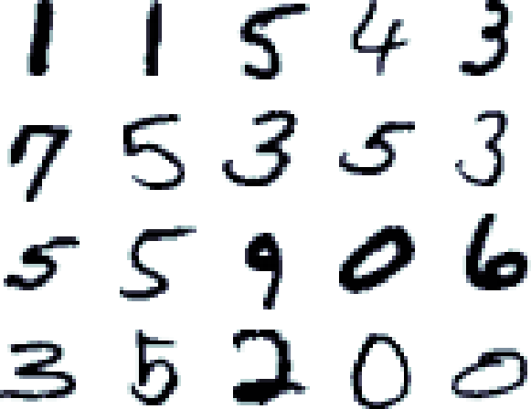
Problem As in CNTK 103B, we will continue to work on the same problem of recognizing digits in MNIST data. The MNIST data comprises hand-written digits with little background noise.

# Figure 1
Image(url= "http://3.bp.blogspot.com/_UpN7DfJA0j4/TJtUBWPk0SI/AAAAAAAAABY/oWPMtmqJn3k/s1600/mnist_originals.png", width=200, height=200)

Goal: Our goal is to train a classifier that will identify the digits in the MNIST dataset. Additionally, we aspire to achieve lower error rate with Multi-layer perceptron compared to Multi-class logistic regression.

Approach: The same 5 stages we have used in the previous tutorial are applicable: Data reading, Data preprocessing, Creating a model, Learning the model parameters and Evaluating (a.k.a. testing/prediction) the model. - Data reading: We will use the CNTK Text reader - Data preprocessing: Covered in part A (suggested extension section).

There is a high overlap with CNTK 102. Though this tutorial we adapt the same model to work on MNIST data with 10 classes instead of the 2 classes we used in CNTK 102.

from __future__ import print_function # Use a function definition from future version (say 3.x from 2.7 interpreter)
import matplotlib.image as mpimg
import matplotlib.pyplot as plt
import numpy as np
import sys
import os

import cntk as C
import cntk.tests.test_utils
cntk.tests.test_utils.set_device_from_pytest_env() # (only needed for our build system)
C.cntk_py.set_fixed_random_seed(1) # fix a random seed for CNTK components

%matplotlib inline

Data reading

In this section, we will read the data generated in CNTK 103 Part A.

# Define the data dimensions
input_dim = 784
num_output_classes = 10

In this tutorial we are using the MNIST data you have downloaded using CNTK_103A_MNIST_DataLoader notebook. The dataset has 60,000 training images and 10,000 test images with each image being 28 x 28 pixels. Thus the number of features is equal to 784 (= 28 x 28 pixels), 1 per pixel. The variable num_output_classes is set to 10 corresponding to the number of digits (0-9) in the dataset.

The data is in the following format:

|labels 0 0 0 0 0 0 0 1 0 0 |features 0 0 0 0 ...
                                              (784 integers each representing a pixel)

In this tutorial we are going to use the image pixels corresponding the integer stream named “features”. We define a create_reader function to read the training and test data using the CTF deserializer. The labels are 1-hot encoded. Refer to CNTK 103A tutorial for data format visualizations.

# Read a CTF formatted text (as mentioned above) using the CTF deserializer from a file
def create_reader(path, is_training, input_dim, num_label_classes):
    return C.io.MinibatchSource(C.io.CTFDeserializer(path, C.io.StreamDefs(
        labels = C.io.StreamDef(field='labels', shape=num_label_classes, is_sparse=False),
        features   = C.io.StreamDef(field='features', shape=input_dim, is_sparse=False)
    )), randomize = is_training, max_sweeps = C.io.INFINITELY_REPEAT if is_training else 1)

# Ensure the training and test data is generated and available for this tutorial.
# We search in two locations in the toolkit for the cached MNIST data set.
data_found = False
for data_dir in [os.path.join("..", "Examples", "Image", "DataSets", "MNIST"),
                 os.path.join("data", "MNIST")]:
    train_file = os.path.join(data_dir, "Train-28x28_cntk_text.txt")
    test_file = os.path.join(data_dir, "Test-28x28_cntk_text.txt")
    if os.path.isfile(train_file) and os.path.isfile(test_file):
        data_found = True
        break
if not data_found:
    raise ValueError("Please generate the data by completing CNTK 103 Part A")
print("Data directory is {0}".format(data_dir))

Data directory is ..\Examples\Image\DataSets\MNIST

Model Creation

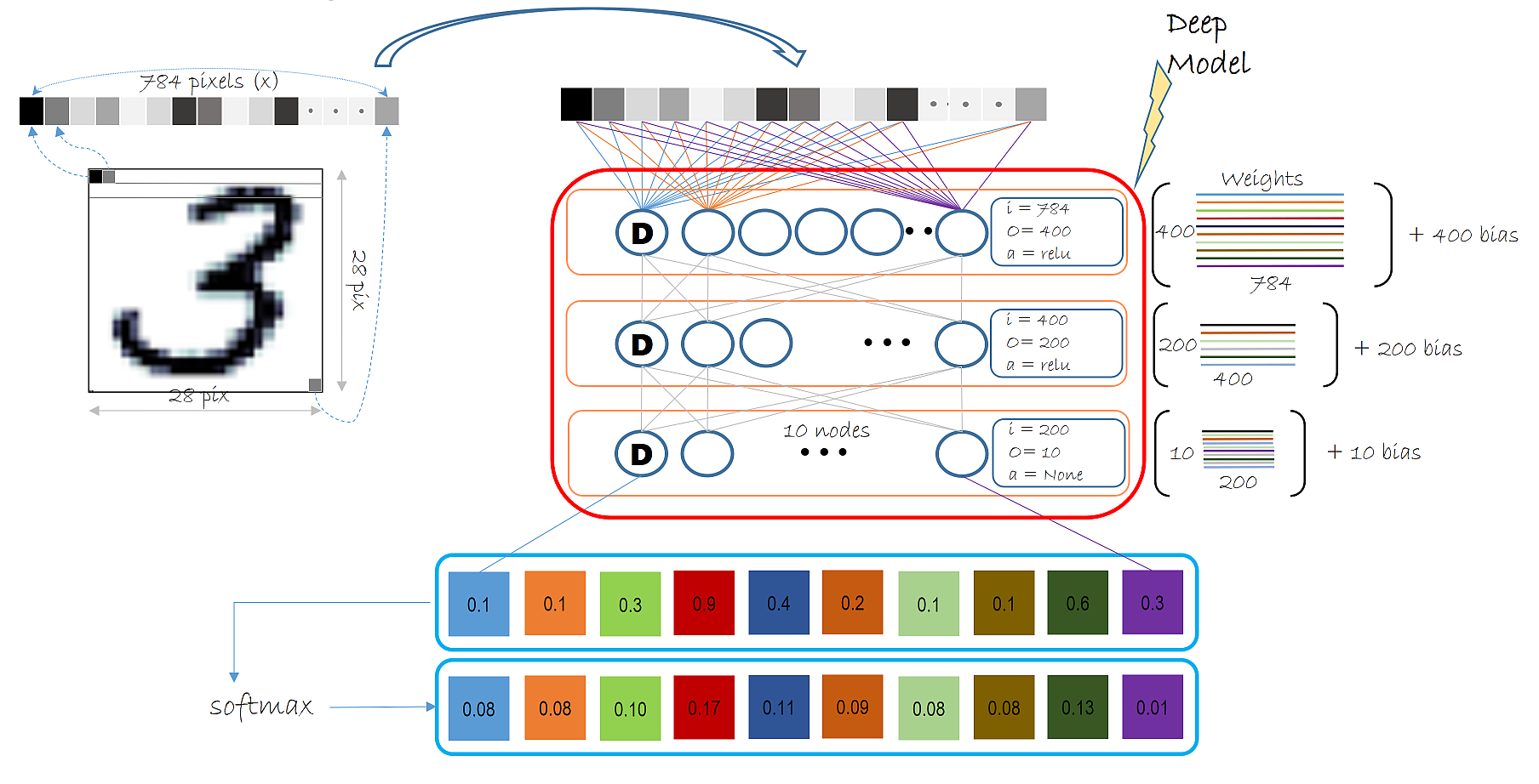
Our multi-layer perceptron will be relatively simple with 2 hidden layers (num_hidden_layers). The number of nodes in the hidden layer being a parameter specified by hidden_layers_dim. The figure below illustrates the entire model we will use in this tutorial in the context of MNIST data.

If you are not familiar with the terms hidden layer and number of hidden layers, please refer back to CNTK 102 tutorial.

Each Dense layer (as illustrated below) shows the input dimensions, output dimensions and activation function that layer uses. Specifically, the layer below shows: input dimension = 784 (1 dimension for each input pixel), output dimension = 400 (number of hidden nodes, a parameter specified by the user) and activation function being relu.

In this model we have 2 dense layer called the hidden layers each with an activation function of relu and one output layer with no activation.

The output dimension (a.k.a. number of hidden nodes) in the 2 hidden layer is set to 400 and 200 in the illustration above. In the code below we keep both layers to have the same number of hidden nodes (set to 400). The number of hidden layers is 2. Fill in the following values: - num_hidden_layers - hidden_layers_dim

The final output layer emits a vector of 10 values. Since we will be using softmax to normalize the output of the model we do not use an activation function in this layer. The softmax operation comes bundled with the loss function we will be using later in this tutorial.

num_hidden_layers = 2
hidden_layers_dim = 400

Network input and output: - input variable (a key CNTK concept): >An input variable is a container in which we fill different observations in this case image pixels during model learning (a.k.a.training) and model evaluation (a.k.a. testing). Thus, the shape of the input must match the shape of the data that will be provided. For example, when data are images each of height 10 pixels and width 5 pixels, the input feature dimension will be 50 (representing the total number of image pixels). More on data and their dimensions to appear in separate tutorials.

Question What is the input dimension of your chosen model? This is fundamental to our understanding of variables in a network or model representation in CNTK.

input = C.input_variable(input_dim)
label = C.input_variable(num_output_classes)

Multi-layer Perceptron setup

The cell below is a direct translation of the illustration of the model shown above.

def create_model(features):
    with C.layers.default_options(init = C.layers.glorot_uniform(), activation = C.ops.relu):
            h = features
            for _ in range(num_hidden_layers):
                h = C.layers.Dense(hidden_layers_dim)(h)
            r = C.layers.Dense(num_output_classes, activation = None)(h)
            return r

z = create_model(input)

z will be used to represent the output of a network.

We introduced sigmoid function in CNTK 102, in this tutorial you should try different activation functions in the hidden layer. You may choose to do this right away and take a peek into the performance later in the tutorial or run the preset tutorial and then choose to perform the suggested activity.

** Suggested Activity ** - Record the training error you get with sigmoid as the activation function - Now change to relu as the activation function and see if you can improve your training error

Quiz: Name some of the different supported activation functions. Which activation function gives the least training error?

# Scale the input to 0-1 range by dividing each pixel by 255.
z = create_model(input/255.0)

Learning model parameters

Same as the previous tutorial, we use the softmax function to map the accumulated evidences or activations to a probability distribution over the classes (Details of the softmax function).

Training

Similar to CNTK 102, we minimize the cross-entropy between the label and predicted probability by the network. If this terminology sounds strange to you, please refer to the tutorial CNTK 102 for a refresher.

loss = C.cross_entropy_with_softmax(z, label)

Evaluation

In order to evaluate the classification, one can compare the output of the network which for each observation emits a vector of evidences (can be converted into probabilities using softmax functions) with dimension equal to number of classes.

label_error = C.classification_error(z, label)

Configure training

The trainer strives to reduce the loss function by different optimization approaches, Stochastic Gradient Descent (sgd) being a basic one. Typically, one would start with random initialization of the model parameters. The sgd optimizer would calculate the loss or error between the predicted label against the corresponding ground-truth label and using gradient-decent generate a new set model parameters in a single iteration.

The aforementioned model parameter update using a single observation at a time is attractive since it does not require the entire data set (all observation) to be loaded in memory and also requires gradient computation over fewer datapoints, thus allowing for training on large data sets. However, the updates generated using a single observation sample at a time can vary wildly between iterations. An intermediate ground is to load a small set of observations and use an average of the loss or error from that set to update the model parameters. This subset is called a minibatch.

With minibatches we often sample observation from the larger training dataset. We repeat the process of model parameters update using different combination of training samples and over a period of time minimize the loss (and the error). When the incremental error rates are no longer changing significantly or after a preset number of maximum minibatches to train, we claim that our model is trained.

One of the key parameter for optimization is called the learning_rate. For now, we can think of it as a scaling factor that modulates how much we change the parameters in any iteration. We will be covering more details in later tutorial. With this information, we are ready to create our trainer.

# Instantiate the trainer object to drive the model training
learning_rate = 0.2
lr_schedule = C.learning_parameter_schedule(learning_rate)
learner = C.sgd(z.parameters, lr_schedule)
trainer = C.Trainer(z, (loss, label_error), [learner])

First let us create some helper functions that will be needed to visualize different functions associated with training.

# Define a utility function to compute the moving average sum.
# A more efficient implementation is possible with np.cumsum() function
def moving_average(a, w=5):
    if len(a) < w:
        return a[:]    # Need to send a copy of the array
    return [val if idx < w else sum(a[(idx-w):idx])/w for idx, val in enumerate(a)]


# Defines a utility that prints the training progress
def print_training_progress(trainer, mb, frequency, verbose=1):
    training_loss = "NA"
    eval_error = "NA"

    if mb%frequency == 0:
        training_loss = trainer.previous_minibatch_loss_average
        eval_error = trainer.previous_minibatch_evaluation_average
        if verbose:
            print ("Minibatch: {0}, Loss: {1:.4f}, Error: {2:.2f}%".format(mb, training_loss, eval_error*100))

    return mb, training_loss, eval_error

Run the trainer

We are now ready to train our fully connected neural net. We want to decide what data we need to feed into the training engine.

In this example, each iteration of the optimizer will work on minibatch_size sized samples. We would like to train on all 60000 observations. Additionally we will make multiple passes through the data specified by the variable num_sweeps_to_train_with. With these parameters we can proceed with training our simple multi-layer perceptron network.

# Initialize the parameters for the trainer
minibatch_size = 64
num_samples_per_sweep = 60000
num_sweeps_to_train_with = 10
num_minibatches_to_train = (num_samples_per_sweep * num_sweeps_to_train_with) / minibatch_size

# Create the reader to training data set
reader_train = create_reader(train_file, True, input_dim, num_output_classes)

# Map the data streams to the input and labels.
input_map = {
    label  : reader_train.streams.labels,
    input  : reader_train.streams.features
}

# Run the trainer on and perform model training
training_progress_output_freq = 500

plotdata = {"batchsize":[], "loss":[], "error":[]}

for i in range(0, int(num_minibatches_to_train)):

    # Read a mini batch from the training data file
    data = reader_train.next_minibatch(minibatch_size, input_map = input_map)

    trainer.train_minibatch(data)
    batchsize, loss, error = print_training_progress(trainer, i, training_progress_output_freq, verbose=1)

    if not (loss == "NA" or error =="NA"):
        plotdata["batchsize"].append(batchsize)
        plotdata["loss"].append(loss)
        plotdata["error"].append(error)

Minibatch: 0, Loss: 2.3106, Error: 81.25%
Minibatch: 500, Loss: 0.2747, Error: 7.81%
Minibatch: 1000, Loss: 0.0964, Error: 1.56%
Minibatch: 1500, Loss: 0.1252, Error: 4.69%
Minibatch: 2000, Loss: 0.0086, Error: 0.00%
Minibatch: 2500, Loss: 0.0387, Error: 1.56%
Minibatch: 3000, Loss: 0.0206, Error: 0.00%
Minibatch: 3500, Loss: 0.0486, Error: 3.12%
Minibatch: 4000, Loss: 0.0178, Error: 0.00%
Minibatch: 4500, Loss: 0.0107, Error: 0.00%
Minibatch: 5000, Loss: 0.0077, Error: 0.00%
Minibatch: 5500, Loss: 0.0042, Error: 0.00%
Minibatch: 6000, Loss: 0.0045, Error: 0.00%
Minibatch: 6500, Loss: 0.0292, Error: 0.00%
Minibatch: 7000, Loss: 0.0190, Error: 1.56%
Minibatch: 7500, Loss: 0.0060, Error: 0.00%
Minibatch: 8000, Loss: 0.0031, Error: 0.00%
Minibatch: 8500, Loss: 0.0019, Error: 0.00%
Minibatch: 9000, Loss: 0.0006, Error: 0.00%

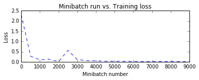
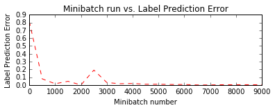
Let us plot the errors over the different training minibatches. Note that as we iterate the training loss decreases though we do see some intermediate bumps.

Hence, we use smaller minibatches and using sgd enables us to have a great scalability while being performant for large data sets. There are advanced variants of the optimizer unique to CNTK that enable harnessing computational efficiency for real world data sets and will be introduced in advanced tutorials.

# Compute the moving average loss to smooth out the noise in SGD
plotdata["avgloss"] = moving_average(plotdata["loss"])
plotdata["avgerror"] = moving_average(plotdata["error"])

# Plot the training loss and the training error
import matplotlib.pyplot as plt

plt.figure(1)
plt.subplot(211)
plt.plot(plotdata["batchsize"], plotdata["avgloss"], 'b--')
plt.xlabel('Minibatch number')
plt.ylabel('Loss')
plt.title('Minibatch run vs. Training loss')

plt.show()

plt.subplot(212)
plt.plot(plotdata["batchsize"], plotdata["avgerror"], 'r--')
plt.xlabel('Minibatch number')
plt.ylabel('Label Prediction Error')
plt.title('Minibatch run vs. Label Prediction Error')
plt.show()

Run evaluation / testing

Now that we have trained the network, let us evaluate the trained network on the test data. This is done using trainer.test_minibatch.

# Read the training data
reader_test = create_reader(test_file, False, input_dim, num_output_classes)

test_input_map = {
    label  : reader_test.streams.labels,
    input  : reader_test.streams.features,
}

# Test data for trained model
test_minibatch_size = 512
num_samples = 10000
num_minibatches_to_test = num_samples // test_minibatch_size
test_result = 0.0

for i in range(num_minibatches_to_test):

    # We are loading test data in batches specified by test_minibatch_size
    # Each data point in the minibatch is a MNIST digit image of 784 dimensions
    # with one pixel per dimension that we will encode / decode with the
    # trained model.
    data = reader_test.next_minibatch(test_minibatch_size,
                                      input_map = test_input_map)

    eval_error = trainer.test_minibatch(data)
    test_result = test_result + eval_error

# Average of evaluation errors of all test minibatches
print("Average test error: {0:.2f}%".format(test_result*100 / num_minibatches_to_test))

Average test error: 1.74%

Note, this error is very comparable to our training error indicating that our model has good “out of sample” error a.k.a. generalization error. This implies that our model can very effectively deal with previously unseen observations (during the training process). This is key to avoid the phenomenon of overfitting.

Huge reduction in error compared to multi-class LR (from CNTK 103B).

We have so far been dealing with aggregate measures of error. Let us now get the probabilities associated with individual data points. For each observation, the eval function returns the probability distribution across all the classes. The classifier is trained to recognize digits, hence has 10 classes. First let us route the network output through a softmax function. This maps the aggregated activations across the network to probabilities across the 10 classes.

out = C.softmax(z)

Let us a small minibatch sample from the test data.

# Read the data for evaluation
reader_eval = create_reader(test_file, False, input_dim, num_output_classes)

eval_minibatch_size = 25
eval_input_map = {input: reader_eval.streams.features}

data = reader_test.next_minibatch(eval_minibatch_size, input_map = test_input_map)

img_label = data[label].asarray()
img_data = data[input].asarray()
predicted_label_prob = [out.eval(img_data[i]) for i in range(len(img_data))]

# Find the index with the maximum value for both predicted as well as the ground truth
pred = [np.argmax(predicted_label_prob[i]) for i in range(len(predicted_label_prob))]
gtlabel = [np.argmax(img_label[i]) for i in range(len(img_label))]

print("Label    :", gtlabel[:25])
print("Predicted:", pred)

Label    : [4, 5, 6, 7, 8, 9, 7, 4, 6, 1, 4, 0, 9, 9, 3, 7, 8, 4, 7, 5, 8, 5, 3, 2, 2]
Predicted: [4, 6, 6, 7, 8, 9, 7, 4, 6, 1, 4, 0, 9, 9, 3, 7, 8, 0, 7, 5, 8, 5, 3, 2, 2]

Let us visualize some of the results

# Plot a random image
sample_number = 5
plt.imshow(img_data[sample_number].reshape(28,28), cmap="gray_r")
plt.axis('off')

img_gt, img_pred = gtlabel[sample_number], pred[sample_number]
print("Image Label: ", img_pred)

Image Label:  9

Exploration Suggestion - Try exploring how the classifier behaves with different parameters, e.g. changing the minibatch_size parameter from 25 to say 64 or 128. What happens to the error rate? How does the error compare to the logistic regression classifier? - Try increasing the number of sweeps - Can you change the network to reduce the training error rate? When do you see overfitting happening?

Code link

If you want to try running the tutorial from Python command prompt please run the SimpleMNIST.py example.