In [1]:
from IPython.display import Image
CNTK 201: Part B - Image Understanding
This tutorial shows how to implement image recognition task using convolution network with CNTK v2 Python API. You will start with a basic feedforward CNN architecture to classify CIFAR dataset, then you will keep adding advanced features to your network. Finally, you will implement a VGG net and residual net like the one that won ImageNet competition but smaller in size.
Introduction
In this tutorial, you will practice the following:
- Understanding subset of CNTK python API needed for image classification task.
- Write a custom convolution network to classify CIFAR dataset.
- Modifying the network structure by adding:
- Dropout layer.
- Batchnormalization layer.
- Implement a VGG style network.
- Introduction to Residual Nets (RESNET).
- Implement and train RESNET network.
Prerequisites
Please run CNTK 201A image data downloader notebook to download and prepare CIFAR dataset.
CNTK 102 lab is recommended but not a prerequisite for this tutorial. However, a basic understanding of Deep Learning is needed. Familiarity with basic convolution operations is highly desirable (Refer to CNTK tutorial 103D).
Dataset
You will use CIFAR 10 dataset, from https://www.cs.toronto.edu/~kriz/cifar.html, during this tutorial. The dataset contains 50000 training images and 10000 test images, all images are 32 x 32 x 3. Each image is classified as one of 10 classes as shown below:
In [2]:
# Figure 1
Image(url="https://cntk.ai/jup/201/cifar-10.png", width=500, height=500)
Out[2]:
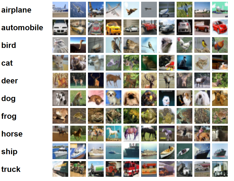
The above image is from: https://www.cs.toronto.edu/~kriz/cifar.html
Convolution Neural Network (CNN)
We recommend completing CNTK 103D tutorial before proceeding. Here is a brief recap of Convolution Neural Network (CNN). CNN is a feedforward network comprise of a bunch of layers in such a way that the output of one layer is fed to the next layer (There are more complex architecture that skip layers, we will discuss one of those at the end of this lab). Usually, CNN start with alternating between convolution layer and pooling layer (downsample), then end up with fully connected layer for the classification part.
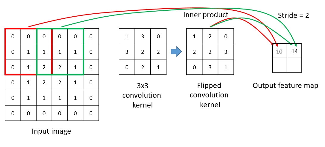
Convolution layer
Convolution layer consist of multiple 2D convolution kernels applied on the input image or the previous layer, each convolution kernel outputs a feature map.
In [3]:
# Figure 2
Image(url="https://cntk.ai/jup/201/Conv2D.png")
Out[3]:
The stack of feature maps output are the input to the next layer.
In [4]:
# Figure 3
Image(url="https://cntk.ai/jup/201/Conv2DFeatures.png")
Out[4]:
In CNTK:
Here the convolution layer in Python:
def Convolution(filter_shape,        # e.g. (3,3)
                num_filters,         # e.g. 64
                activation,          # relu or None...etc.
                init,                # Random initialization
                pad,                 # True or False
                strides)             # strides e.g. (1,1)
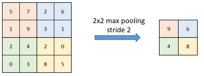
Pooling layer
In most CNN vision architecture, each convolution layer is succeeded by a pooling layer, so they keep alternating until the fully connected layer.
The purpose of the pooling layer is as follow:
- Reduce the dimensionality of the previous layer, which speed up the network.
- Provide a limited translation invariant.
Here an example of max pooling with a stride of 2:
In [5]:
# Figure 4
Image(url="https://cntk.ai/jup/201/MaxPooling.png", width=400, height=400)
Out[5]:
In CNTK:
Here the pooling layer in Python:
# Max pooling
def MaxPooling(filter_shape,  # e.g. (3,3)
               strides,       # (2,2)
               pad)           # True or False

# Average pooling
def AveragePooling(filter_shape,  # e.g. (3,3)
                   strides,       # (2,2)
                   pad)           # True or False
Dropout layer
Dropout layer takes a probability value as an input, the value is called the dropout rate. Let us say the dropout rate is 0.5, what this layer does it pick at random 50% of the nodes from the previous layer and drop them out of the network. This behavior help regularize the network.
Dropout: A Simple Way to Prevent Neural Networks from Overfitting Nitish Srivastava, Geoffrey Hinton, Alex Krizhevsky, Ilya Sutskever, Ruslan Salakhutdinov
In CNTK:
Dropout layer in Python:
# Dropout
def Dropout(prob)    # dropout rate e.g. 0.5
Batch normalization (BN)
Batch normalization is a way to make the input to each layer has zero mean and unit variance. BN help the network converge faster and keep the input of each layer around zero. BN has two learnable parameters called gamma and beta, the purpose of those parameters is for the network to decide for itself if the normalized input is what is best or the raw input.
Batch Normalization: Accelerating Deep Network Training by Reducing Internal Covariate Shift Sergey Ioffe, Christian Szegedy
In CNTK:
Batch normalization layer in Python:
# Batch normalization
def BatchNormalization(map_rank)  # For image map_rank=1
Let us begin by first importing the modules.
In [6]:
from __future__ import print_function # Use a function definition from future version (say 3.x from 2.7 interpreter)

import matplotlib.pyplot as plt
import math
import numpy as np
import os
import PIL
import sys
try:
    from urllib.request import urlopen
except ImportError:
    from urllib import urlopen

import cntk as C
In the block below, we check if we are running this notebook in the CNTK internal test machines by looking for environment variables defined there. We then select the right target device (GPU vs CPU) to test this notebook. In other cases, we use CNTK’s default policy to use the best available device (GPU, if available, else CPU).
In [7]:
if 'TEST_DEVICE' in os.environ:
    if os.environ['TEST_DEVICE'] == 'cpu':
        C.device.try_set_default_device(C.device.cpu())
    else:
        C.device.try_set_default_device(C.device.gpu(0))
Data reading
To train the above model we need two things: * Read the training images and their corresponding labels. * Define a cost function, compute the cost for each mini-batch and update the model weights according to the cost value.
To read the data in CNTK, we will use CNTK readers which handle data augmentation and can fetch data in parallel.
Example of a map text file:
S:\data\CIFAR-10\train\00001.png    9
S:\data\CIFAR-10\train\00002.png    9
S:\data\CIFAR-10\train\00003.png    4
S:\data\CIFAR-10\train\00004.png    1
S:\data\CIFAR-10\train\00005.png    1
In [10]:
# Determine the data path for testing
# Check for an environment variable defined in CNTK's test infrastructure
envvar = 'CNTK_EXTERNAL_TESTDATA_SOURCE_DIRECTORY'
def is_test(): return envvar in os.environ

if is_test():
    data_path = os.path.join(os.environ[envvar],'Image','CIFAR','v0','tutorial201')
    data_path = os.path.normpath(data_path)
else:
    data_path = os.path.join('data', 'CIFAR-10')

# model dimensions
image_height = 32
image_width  = 32
num_channels = 3
num_classes  = 10

import cntk.io.transforms as xforms
#
# Define the reader for both training and evaluation action.
#
def create_reader(map_file, mean_file, train):
    print("Reading map file:", map_file)
    print("Reading mean file:", mean_file)

    if not os.path.exists(map_file) or not os.path.exists(mean_file):
        raise RuntimeError("This tutorials depends 201A tutorials, please run 201A first.")

    # transformation pipeline for the features has jitter/crop only when training
    transforms = []
    # train uses data augmentation (translation only)
    if train:
        transforms += [
            xforms.crop(crop_type='randomside', side_ratio=0.8)
        ]
    transforms += [
        xforms.scale(width=image_width, height=image_height, channels=num_channels, interpolations='linear'),
        xforms.mean(mean_file)
    ]
    # deserializer
    return C.io.MinibatchSource(C.io.ImageDeserializer(map_file, C.io.StreamDefs(
        features = C.io.StreamDef(field='image', transforms=transforms), # first column in map file is referred to as 'image'
        labels   = C.io.StreamDef(field='label', shape=num_classes)      # and second as 'label'
    )))
In [11]:
# Create the train and test readers
reader_train = create_reader(os.path.join(data_path, 'train_map.txt'),
                             os.path.join(data_path, 'CIFAR-10_mean.xml'), True)
reader_test  = create_reader(os.path.join(data_path, 'test_map.txt'),
                             os.path.join(data_path, 'CIFAR-10_mean.xml'), False)
Reading map file: c:\Data\CNTKTestData\Image\CIFAR\v0\tutorial201\train_map.txt
Reading mean file: c:\Data\CNTKTestData\Image\CIFAR\v0\tutorial201\CIFAR-10_mean.xml
Reading map file: c:\Data\CNTKTestData\Image\CIFAR\v0\tutorial201\test_map.txt
Reading mean file: c:\Data\CNTKTestData\Image\CIFAR\v0\tutorial201\CIFAR-10_mean.xml
In [8]:
# Figure 5
Image(url="https://cntk.ai/jup/201/CNN.png")
Out[8]:
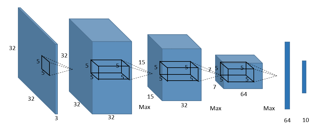
Model creation (Basic CNN)
Now that we imported the needed modules, let’s implement our first CNN, as shown in Figure 5 above.
Let’s implement the above network using CNTK layer API:
In [9]:
def create_basic_model(input, out_dims):
    with C.layers.default_options(init=C.glorot_uniform(), activation=C.relu):
        net = C.layers.Convolution((5,5), 32, pad=True)(input)
        net = C.layers.MaxPooling((3,3), strides=(2,2))(net)

        net = C.layers.Convolution((5,5), 32, pad=True)(net)
        net = C.layers.MaxPooling((3,3), strides=(2,2))(net)

        net = C.layers.Convolution((5,5), 64, pad=True)(net)
        net = C.layers.MaxPooling((3,3), strides=(2,2))(net)

        net = C.layers.Dense(64)(net)
        net = C.layers.Dense(out_dims, activation=None)(net)

    return net
Training and evaluation
Now let us write the training and evaluation loop.
In [12]:
#
# Train and evaluate the network.
#
def train_and_evaluate(reader_train, reader_test, max_epochs, model_func):
# Input variables denoting the features and label data
input_var = C.input_variable((num_channels, image_height, image_width))
label_var = C.input_variable((num_classes))
# Normalize the input
feature_scale = 1.0 / 256.0
input_var_norm = C.element_times(feature_scale, input_var)
# apply model to input
z = model_func(input_var_norm, out_dims=10)
#
# Training action
#
# loss and metric
ce = C.cross_entropy_with_softmax(z, label_var)
pe = C.classification_error(z, label_var)
# training config
epoch_size = 50000
minibatch_size = 64
# Set training parameters
lr_per_minibatch = C.learning_parameter_schedule([0.01]*10 + [0.003]*10 + [0.001],
epoch_size = epoch_size)
momentums = C.momentum_schedule(0.9, minibatch_size = minibatch_size)
l2_reg_weight = 0.001
# trainer object
learner = C.momentum_sgd(z.parameters,
lr = lr_per_minibatch,
momentum = momentums,
l2_regularization_weight=l2_reg_weight)
progress_printer = C.logging.ProgressPrinter(tag='Training', num_epochs=max_epochs)
trainer = C.Trainer(z, (ce, pe), [learner], [progress_printer])
# define mapping from reader streams to network inputs
input_map = {
input_var: reader_train.streams.features,
label_var: reader_train.streams.labels
}
C.logging.log_number_of_parameters(z) ; print()
# perform model training
batch_index = 0
plot_data = {'batchindex':[], 'loss':[], 'error':[]}
for epoch in range(max_epochs): # loop over epochs
sample_count = 0
while sample_count < epoch_size: # loop over minibatches in the epoch
data = reader_train.next_minibatch(min(minibatch_size, epoch_size - sample_count),
input_map=input_map) # fetch minibatch.
trainer.train_minibatch(data) # update model with it
sample_count += data[label_var].num_samples # count samples processed so far
# For visualization...
plot_data['batchindex'].append(batch_index)
plot_data['loss'].append(trainer.previous_minibatch_loss_average)
plot_data['error'].append(trainer.previous_minibatch_evaluation_average)
batch_index += 1
trainer.summarize_training_progress()
#
# Evaluation action
#
epoch_size = 10000
minibatch_size = 16
# process minibatches and evaluate the model
metric_numer = 0
metric_denom = 0
sample_count = 0
minibatch_index = 0
while sample_count < epoch_size:
current_minibatch = min(minibatch_size, epoch_size - sample_count)
# Fetch next test min batch.
data = reader_test.next_minibatch(current_minibatch, input_map=input_map)
# minibatch data to be trained with
metric_numer += trainer.test_minibatch(data) * current_minibatch
metric_denom += current_minibatch
# Keep track of the number of samples processed so far.
sample_count += data[label_var].num_samples
minibatch_index += 1
print("")
print("Final Results: Minibatch[1-{}]: errs = {:0.1f}% * {}".format(minibatch_index+1, (metric_numer*100.0)/metric_denom, metric_denom))
print("")
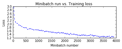
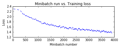
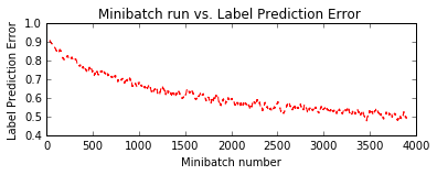
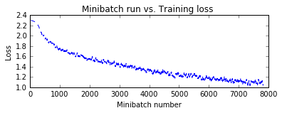
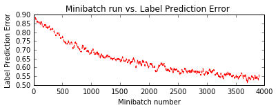
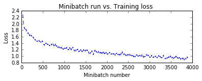
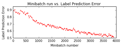
# Visualize training result:
window_width = 32
loss_cumsum = np.cumsum(np.insert(plot_data['loss'], 0, 0))
error_cumsum = np.cumsum(np.insert(plot_data['error'], 0, 0))
# Moving average.
plot_data['batchindex'] = np.insert(plot_data['batchindex'], 0, 0)[window_width:]
plot_data['avg_loss'] = (loss_cumsum[window_width:] - loss_cumsum[:-window_width]) / window_width
plot_data['avg_error'] = (error_cumsum[window_width:] - error_cumsum[:-window_width]) / window_width
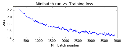
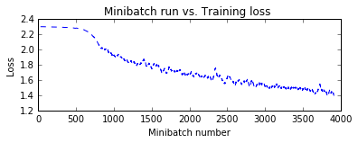
plt.figure(1)
plt.subplot(211)
plt.plot(plot_data["batchindex"], plot_data["avg_loss"], 'b--')
plt.xlabel('Minibatch number')
plt.ylabel('Loss')
plt.title('Minibatch run vs. Training loss ')
plt.show()
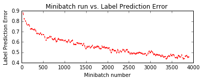
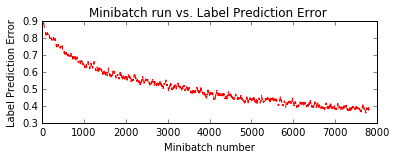
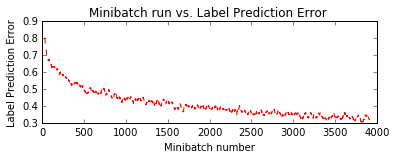
plt.subplot(212)
plt.plot(plot_data["batchindex"], plot_data["avg_error"], 'r--')
plt.xlabel('Minibatch number')
plt.ylabel('Label Prediction Error')
plt.title('Minibatch run vs. Label Prediction Error ')
plt.show()
return C.softmax(z)
In [13]:
pred = train_and_evaluate(reader_train,
                          reader_test,
                          max_epochs=5,
                          model_func=create_basic_model)
Training 116906 parameters in 10 parameter tensors.

Learning rate per minibatch: 0.01
Momentum per sample: 0.9983550962823424
Finished Epoch[1 of 5]: [Training] loss = 2.127933 * 50000, metric = 77.96% * 50000 15.851s (3154.4 samples/s);
Finished Epoch[2 of 5]: [Training] loss = 1.768975 * 50000, metric = 64.90% * 50000 11.970s (4177.1 samples/s);
Finished Epoch[3 of 5]: [Training] loss = 1.589650 * 50000, metric = 58.28% * 50000 11.958s (4181.3 samples/s);
Finished Epoch[4 of 5]: [Training] loss = 1.495402 * 50000, metric = 54.32% * 50000 11.960s (4180.6 samples/s);
Finished Epoch[5 of 5]: [Training] loss = 1.421285 * 50000, metric = 51.41% * 50000 11.965s (4178.9 samples/s);

Final Results: Minibatch[1-626]: errs = 46.4% * 10000
Although, this model is very simple, it still has too much code, we can do better. Here the same model in more terse format:
In [14]:
def create_basic_model_terse(input, out_dims):

    with C.layers.default_options(init=C.glorot_uniform(), activation=C.relu):
        model = C.layers.Sequential([
            C.layers.For(range(3), lambda i: [
                C.layers.Convolution((5,5), [32,32,64][i], pad=True),
                C.layers.MaxPooling((3,3), strides=(2,2))
                ]),
            C.layers.Dense(64),
            C.layers.Dense(out_dims, activation=None)
        ])

    return model(input)
In [15]:
pred_basic_model = train_and_evaluate(reader_train,
                                      reader_test,
                                      max_epochs=10,
                                      model_func=create_basic_model_terse)
Training 116906 parameters in 10 parameter tensors.

Learning rate per minibatch: 0.01
Momentum per sample: 0.9983550962823424
Finished Epoch[1 of 10]: [Training] loss = 2.064481 * 50000, metric = 75.90% * 50000 12.260s (4078.3 samples/s);
Finished Epoch[2 of 10]: [Training] loss = 1.703777 * 50000, metric = 63.17% * 50000 12.127s (4123.0 samples/s);
Finished Epoch[3 of 10]: [Training] loss = 1.561847 * 50000, metric = 57.11% * 50000 12.116s (4126.8 samples/s);
Finished Epoch[4 of 10]: [Training] loss = 1.463862 * 50000, metric = 53.17% * 50000 12.078s (4139.8 samples/s);
Finished Epoch[5 of 10]: [Training] loss = 1.374724 * 50000, metric = 49.49% * 50000 12.117s (4126.4 samples/s);
Finished Epoch[6 of 10]: [Training] loss = 1.294328 * 50000, metric = 46.14% * 50000 12.158s (4112.5 samples/s);
Finished Epoch[7 of 10]: [Training] loss = 1.231594 * 50000, metric = 43.62% * 50000 12.084s (4137.7 samples/s);
Finished Epoch[8 of 10]: [Training] loss = 1.179700 * 50000, metric = 41.84% * 50000 12.156s (4113.2 samples/s);
Finished Epoch[9 of 10]: [Training] loss = 1.136541 * 50000, metric = 39.93% * 50000 12.065s (4144.2 samples/s);
Finished Epoch[10 of 10]: [Training] loss = 1.096253 * 50000, metric = 38.56% * 50000 12.148s (4115.9 samples/s);

Final Results: Minibatch[1-626]: errs = 34.4% * 10000
Now that we have a trained model, let us classify the following image of a truck. We use PIL to read the image.
In [16]:
# Figure 6
Image(url="https://cntk.ai/jup/201/00014.png", width=64, height=64)
Out[16]:

In [17]:
# Download a sample image
# (this is 00014.png from test dataset)
# Any image of size 32,32 can be evaluated

url = "https://cntk.ai/jup/201/00014.png"
myimg = np.array(PIL.Image.open(urlopen(url)), dtype=np.float32)
During training we have subtracted the mean from the input images. Here we take an approximate value of the mean and subtract it from the image.
In [18]:
def eval(pred_op, image_data):
    label_lookup = ["airplane", "automobile", "bird", "cat", "deer", "dog", "frog", "horse", "ship", "truck"]
    image_mean = 133.0
    image_data -= image_mean
    image_data = np.ascontiguousarray(np.transpose(image_data, (2, 0, 1)))

    result = np.squeeze(pred_op.eval({pred_op.arguments[0]:[image_data]}))

    # Return top 3 results:
    top_count = 3
    result_indices = (-np.array(result)).argsort()[:top_count]

    print("Top 3 predictions:")
    for i in range(top_count):
        print("\tLabel: {:10s}, confidence: {:.2f}%".format(label_lookup[result_indices[i]], result[result_indices[i]] * 100))
In [19]:
# Run the evaluation on the downloaded image
eval(pred_basic_model, myimg)
Top 3 predictions:
        Label: truck     , confidence: 96.59%
        Label: ship      , confidence: 2.31%
        Label: cat       , confidence: 0.43%
Model: CNN with dropout
Adding dropout layer, with drop rate of 0.25, before the last dense layer:
In [20]:
def create_basic_model_with_dropout(input, out_dims):

    with C.layers.default_options(activation=C.relu, init=C.glorot_uniform()):
        model = C.layers.Sequential([
            C.layers.For(range(3), lambda i: [
                C.layers.Convolution((5,5), [32,32,64][i], pad=True),
                C.layers.MaxPooling((3,3), strides=(2,2))
            ]),
            C.layers.Dense(64),
            C.layers.Dropout(0.25),
            C.layers.Dense(out_dims, activation=None)
        ])

    return model(input)
In [21]:
pred_basic_model_dropout = train_and_evaluate(reader_train,
                                              reader_test,
                                              max_epochs=5,
                                              model_func=create_basic_model_with_dropout)
Training 116906 parameters in 10 parameter tensors.

Learning rate per minibatch: 0.01
Momentum per sample: 0.9983550962823424
Finished Epoch[1 of 5]: [Training] loss = 2.107245 * 50000, metric = 79.08% * 50000 12.977s (3853.0 samples/s);
Finished Epoch[2 of 5]: [Training] loss = 1.795581 * 50000, metric = 67.10% * 50000 12.244s (4083.6 samples/s);
Finished Epoch[3 of 5]: [Training] loss = 1.657041 * 50000, metric = 61.52% * 50000 12.265s (4076.6 samples/s);
Finished Epoch[4 of 5]: [Training] loss = 1.567592 * 50000, metric = 57.72% * 50000 12.251s (4081.3 samples/s);
Finished Epoch[5 of 5]: [Training] loss = 1.500142 * 50000, metric = 54.97% * 50000 12.228s (4089.0 samples/s);

Final Results: Minibatch[1-626]: errs = 47.1% * 10000
Model: CNN with BN
Add batch normalization after each convolution and before the last dense layer:
In [22]:
def create_basic_model_with_batch_normalization(input, out_dims):

    with C.layers.default_options(activation=C.relu, init=C.glorot_uniform()):
        model = C.layers.Sequential([
            C.layers.For(range(3), lambda i: [
                C.layers.Convolution((5,5), [32,32,64][i], pad=True),
                C.layers.BatchNormalization(map_rank=1),
                C.layers.MaxPooling((3,3), strides=(2,2))
            ]),
            C.layers.Dense(64),
            C.layers.BatchNormalization(map_rank=1),
            C.layers.Dense(out_dims, activation=None)
        ])

    return model(input)
In [23]:
pred_basic_model_bn = train_and_evaluate(reader_train,
                                         reader_test,
                                         max_epochs=5,
                                         model_func=create_basic_model_with_batch_normalization)
Training 117290 parameters in 18 parameter tensors.

Learning rate per minibatch: 0.01
Momentum per sample: 0.9983550962823424
Finished Epoch[1 of 5]: [Training] loss = 1.536584 * 50000, metric = 55.22% * 50000 12.978s (3852.7 samples/s);
Finished Epoch[2 of 5]: [Training] loss = 1.215455 * 50000, metric = 43.35% * 50000 12.196s (4099.7 samples/s);
Finished Epoch[3 of 5]: [Training] loss = 1.092067 * 50000, metric = 38.66% * 50000 12.260s (4078.3 samples/s);
Finished Epoch[4 of 5]: [Training] loss = 1.011021 * 50000, metric = 35.57% * 50000 12.330s (4055.2 samples/s);
Finished Epoch[5 of 5]: [Training] loss = 0.952613 * 50000, metric = 33.38% * 50000 12.286s (4069.7 samples/s);

Final Results: Minibatch[1-626]: errs = 30.1% * 10000
Popular Model
VGG style network
Let’s implement an inspired VGG style network, using layer API, here the architecture:
| VGG9 |
|---|
| conv3-64 |
| conv3-64 |
| max3 |
| conv3-96 |
| conv3-96 |
| max3 |
| conv3-128 |
| conv3-128 |
| max3 |
| FC-1024 |
| FC-1024 |
| FC-10 |
In [24]:
def create_vgg9_model(input, out_dims):
    with C.layers.default_options(activation=C.relu, init=C.glorot_uniform()):
        model = C.layers.Sequential([
            C.layers.For(range(3), lambda i: [
                C.layers.Convolution((3,3), [64,96,128][i], pad=True),
                C.layers.Convolution((3,3), [64,96,128][i], pad=True),
                C.layers.MaxPooling((3,3), strides=(2,2))
            ]),
            C.layers.For(range(2), lambda : [
                C.layers.Dense(1024)
            ]),
            C.layers.Dense(out_dims, activation=None)
        ])

    return model(input)
In [25]:
pred_vgg = train_and_evaluate(reader_train,
                              reader_test,
                              max_epochs=5,
                              model_func=create_vgg9_model)
Training 2675978 parameters in 18 parameter tensors.

Learning rate per minibatch: 0.01
Momentum per sample: 0.9983550962823424
Finished Epoch[1 of 5]: [Training] loss = 2.267064 * 50000, metric = 84.67% * 50000 18.672s (2677.8 samples/s);
Finished Epoch[2 of 5]: [Training] loss = 1.877782 * 50000, metric = 69.81% * 50000 12.578s (3975.2 samples/s);
Finished Epoch[3 of 5]: [Training] loss = 1.689757 * 50000, metric = 63.07% * 50000 12.729s (3928.0 samples/s);
Finished Epoch[4 of 5]: [Training] loss = 1.564912 * 50000, metric = 57.57% * 50000 12.536s (3988.5 samples/s);
Finished Epoch[5 of 5]: [Training] loss = 1.475126 * 50000, metric = 53.79% * 50000 13.171s (3796.2 samples/s);

Final Results: Minibatch[1-626]: errs = 50.1% * 10000
Residual Network (ResNet)
One of the main problem of a Deep Neural Network is how to propagate the error all the way to the first layer. For a deep network, the gradients keep getting smaller until it has no effect on the network weights. ResNet was designed to overcome such problem, by defining a block with identity path, as shown below:
In [26]:
# Figure 7
Image(url="https://cntk.ai/jup/201/ResNetBlock2.png")
Out[26]:
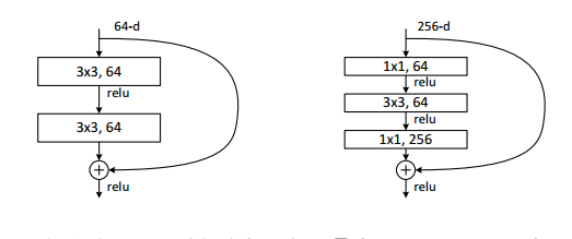
The idea of the above block is 2 folds:
- During back propagation the gradients have a path that does not affect its magnitude.
- The network need to learn residual mapping (delta to x).
So let’s implements ResNet blocks using CNTK:
        ResNetNode                   ResNetNodeInc
            |                              |
     +------+------+             +---------+----------+
     |             |             |                    |
     V             |             V                    V
+----------+       |      +--------------+   +----------------+
| Conv, BN |       |      | Conv x 2, BN |   | SubSample, BN  |
+----------+       |      +--------------+   +----------------+
     |             |             |                    |
     V             |             V                    |
 +-------+         |         +-------+                |
 | ReLU  |         |         | ReLU  |                |
 +-------+         |         +-------+                |
     |             |             |                    |
     V             |             V                    |
+----------+       |        +----------+              |
| Conv, BN |       |        | Conv, BN |              |
+----------+       |        +----------+              |
     |             |             |                    |
     |    +---+    |             |       +---+        |
     +--->| + |<---+             +------>+ + +<-------+
          +---+                          +---+
            |                              |
            V                              V
        +-------+                      +-------+
        | ReLU  |                      | ReLU  |
        +-------+                      +-------+
            |                              |
            V                              V
In [27]:
def convolution_bn(input, filter_size, num_filters, strides=(1,1), init=C.he_normal(), activation=C.relu):
    if activation is None:
        activation = lambda x: x

    r = C.layers.Convolution(filter_size,
                             num_filters,
                             strides=strides,
                             init=init,
                             activation=None,
                             pad=True, bias=False)(input)
    r = C.layers.BatchNormalization(map_rank=1)(r)
    r = activation(r)

    return r

def resnet_basic(input, num_filters):
    c1 = convolution_bn(input, (3,3), num_filters)
    c2 = convolution_bn(c1, (3,3), num_filters, activation=None)
    p  = c2 + input
    return C.relu(p)

def resnet_basic_inc(input, num_filters):
    c1 = convolution_bn(input, (3,3), num_filters, strides=(2,2))
    c2 = convolution_bn(c1, (3,3), num_filters, activation=None)

    s = convolution_bn(input, (1,1), num_filters, strides=(2,2), activation=None)

    p = c2 + s
    return C.relu(p)

def resnet_basic_stack(input, num_filters, num_stack):
    assert (num_stack > 0)

    r = input
    for _ in range(num_stack):
        r = resnet_basic(r, num_filters)
    return r
Let’s write the full model:
In [28]:
def create_resnet_model(input, out_dims):
    conv = convolution_bn(input, (3,3), 16)
    r1_1 = resnet_basic_stack(conv, 16, 3)

    r2_1 = resnet_basic_inc(r1_1, 32)
    r2_2 = resnet_basic_stack(r2_1, 32, 2)

    r3_1 = resnet_basic_inc(r2_2, 64)
    r3_2 = resnet_basic_stack(r3_1, 64, 2)

    # Global average pooling
    pool = C.layers.AveragePooling(filter_shape=(8,8), strides=(1,1))(r3_2)
    net = C.layers.Dense(out_dims, init=C.he_normal(), activation=None)(pool)

    return net
In [29]:
pred_resnet = train_and_evaluate(reader_train, reader_test, max_epochs=5, model_func=create_resnet_model)
Training 272474 parameters in 65 parameter tensors.

Learning rate per minibatch: 0.01
Momentum per sample: 0.9983550962823424
Finished Epoch[1 of 5]: [Training] loss = 1.895607 * 50000, metric = 70.00% * 50000 24.547s (2036.9 samples/s);
Finished Epoch[2 of 5]: [Training] loss = 1.594962 * 50000, metric = 59.18% * 50000 21.075s (2372.5 samples/s);
Finished Epoch[3 of 5]: [Training] loss = 1.456406 * 50000, metric = 53.31% * 50000 21.631s (2311.5 samples/s);
Finished Epoch[4 of 5]: [Training] loss = 1.354717 * 50000, metric = 49.36% * 50000 20.848s (2398.3 samples/s);
Finished Epoch[5 of 5]: [Training] loss = 1.275108 * 50000, metric = 45.98% * 50000 21.164s (2362.5 samples/s);

Final Results: Minibatch[1-626]: errs = 43.9% * 10000