from IPython.display import Image

CNTK 203: Reinforcement Learning Basics

Reinforcement learning (RL) is an area of machine learning inspired by behaviorist psychology, concerned with how software agents ought to take actions in an environment so as to maximize some notion of cumulative reward. In machine learning, the environment is typically formulated as a Markov decision process (MDP) as many reinforcement learning algorithms for this context utilize dynamic programming techniques.

In some machine learning settings, we do not have immediate access to labels, so we cannot rely on supervised learning techniques. If, however, there is something we can interact with and thereby get some feedback that tells us occasionally, whether our previous behavior was good or not, we can use RL to learn how to improve our behavior.

Unlike in supervised learning, in RL, labeled correct input/output pairs are never presented and sub-optimal actions are never explicitly corrected. This mimics many of the online learning paradigms which involves finding a balance between exploration (of conditions or actions never learnt before) and exploitation (of already learnt conditions or actions from previous encounters). Multi-arm bandit problems is one of the category of RL algorithms where exploration vs. exploitation trade-off have been thoroughly studied. See figure below for reference.

# Figure 1
Image(url="https://cntk.ai/jup/polecart.gif", width=300, height=300)

Problem

We will use the CartPole environment from OpenAI’s gym simulator to teach a cart to balance a pole. As described in the link above, in the CartPole example, a pole is attached by an un-actuated joint to a cart, which moves along a frictionless track. The system is controlled by applying a force of +1 or -1 to the cart. A reward of +1 is provided for every timestep that the pole remains upright. The episode ends when the pole is more than 15 degrees from vertical, or the cart moves more than 2.4 units from the center. See figure below for reference.

Goal

Our goal is to prevent the pole from falling over as the cart moves with the pole in upright position (perpendicular to the cart) as the starting state. More specifically if the pole is less than 15 degrees from vertical while the cart is within 2.4 units of the center we will collect reward. In this tutorial, we will train till we learn a set of actions (policies) that lead to an average reward of 200 or more over last 50 batches.

In, RL terminology, the goal is to find policies $a$, that maximize the reward $r$ (feedback) through interaction with some environment (in this case the pole being balanced on the cart). So given a series of experiences

$$s \xrightarrow{a} r, s'$$

we then can learn how to choose action $a$ in a given state $s$ to maximize the accumulated reward $r$ over time:

$$Q(s,a) = r_0 + \gamma r_1 + \gamma^2 r_2 + \ldots = r_0 + \gamma \max_a Q^*(s',a)$$

where $\gamma \in [0,1)$ is the discount factor that controls how much we should value reward that is further away. This is called the *Bellmann*-equation.

In this tutorial we will show how to model the state space, how to use the received reward to figure out which action yields the highest future reward.

We present two different popular approaches here:

Deep Q-Networks: DQNs have become famous in 2015 when they were successfully used to train how to play Atari just form raw pixels. We train neural network to learn the $Q(s,a)$ values (thus $Q$-Network ). From these $Q$ functions values we choose the best action.

Policy gradient: This method directly estimates the policy (set of actions) in the network. The outcome is a learning of an ordered set of actions which leads to maximize reward by probabilistically choosing a subset of actions. In this tutorial, we learn the actions using a gradient descent approach to learn the policies.

In this tutorial, we focus how to implement RL in CNTK. We choose a straight forward shallow network. One can extend the approaches by replacing our shallow model with deeper networks that are introduced in other CNTK tutorials.

Additionally, this tutorial is in its early stages and will be evolving in future updates.

Prerequisites

Please run the following cell from the menu above or select the cell below and hit Shift + Enter to ensure the environment is ready. Verify that the following imports work in your notebook.

from __future__ import print_function
from __future__ import division
import matplotlib.pyplot as plt
from matplotlib import style
import numpy as np
import pandas as pd
import seaborn as sns

style.use('ggplot')
%matplotlib inline

We use the following construct to install the OpenAI gym package if it is not installed. For users new to Jupyter environment, this construct can be used to install any python package.

try:
    import gym
except:
    !pip install gym
    import gym

Collecting gym
  Downloading gym-0.9.4.tar.gz (157kB)
Requirement already satisfied: numpy>=1.10.4 in c:\local\anaconda3-4.1.1-windows-x86_64\envs\cntk-py35\lib\site-packages (from gym)
Requirement already satisfied: requests>=2.0 in c:\local\anaconda3-4.1.1-windows-x86_64\envs\cntk-py35\lib\site-packages (from gym)
Requirement already satisfied: six in c:\local\anaconda3-4.1.1-windows-x86_64\envs\cntk-py35\lib\site-packages (from gym)
Collecting pyglet>=1.2.0 (from gym)
  Using cached pyglet-1.2.4-py3-none-any.whl
Requirement already satisfied: certifi>=2017.4.17 in c:\local\anaconda3-4.1.1-windows-x86_64\envs\cntk-py35\lib\site-packages (from requests>=2.0->gym)
Requirement already satisfied: urllib3<1.23,>=1.21.1 in c:\local\anaconda3-4.1.1-windows-x86_64\envs\cntk-py35\lib\site-packages (from requests>=2.0->gym)
Requirement already satisfied: idna<2.7,>=2.5 in c:\local\anaconda3-4.1.1-windows-x86_64\envs\cntk-py35\lib\site-packages (from requests>=2.0->gym)
Requirement already satisfied: chardet<3.1.0,>=3.0.2 in c:\local\anaconda3-4.1.1-windows-x86_64\envs\cntk-py35\lib\site-packages (from requests>=2.0->gym)
Building wheels for collected packages: gym
  Running setup.py bdist_wheel for gym: started
  Running setup.py bdist_wheel for gym: finished with status 'done'
  Stored in directory: C:\Users\yuqtang\AppData\Local\pip\Cache\wheels\ad\46\5a\1833d0ef8149a50e78fdb24a41f47e22a7f4a9dcd649b8db53
Successfully built gym
Installing collected packages: pyglet, gym
Successfully installed gym-0.9.4 pyglet-1.2.4

Select the notebook run mode

There are two run modes: - Fast mode: isFast is set to True. This is the default mode for the notebooks, which means we train for fewer iterations or train / test on limited data. This ensures functional correctness of the notebook though the models produced are far from what a completed training would produce.

• Slow mode: We recommend the user to set this flag to False once the user has gained familiarity with the notebook content and wants to gain insight from running the notebooks for a longer period with different parameters for training.

isFast = True

CartPole: Data and Environment

We will use the CartPole environment from OpenAI’s gym simulator to teach a cart to balance a pole. Please follow the links to get more details.

In every time step, the agent * gets an observation $(x, \dot{x}, \theta, \dot{\theta})$, corresponding to cart position, cart velocity, pole angle with the vertical, pole angular velocity, * performs an action LEFT or RIGHT, and * receives * a reward of +1 for having survived another time step, and * a new state $(x', \dot{x}', \theta', \dot{\theta}')$

The episode ends, if * the pole is more than 15 degrees from vertical and/or * the cart is moving more than 2.4 units from center.

The task is considered done, if * the agent achieved and averaged reward of 200 over the last 50 episodes (if you manage to get a reward of 200 averaged over the last 100 episode you can consider submitting it to OpenAI).

In fast mode these targets are relaxed.

Part 1: DQN

After a transition $(s,a,r,s')$, we are trying to move our value function $Q(s,a)$ closer to our target $r+\gamma \max_{a'}Q(s',a')$, where $\gamma$ is a discount factor for future rewards and ranges in value between 0 and 1.

DQNs * learn the Q-function that maps observation (state, action) to a score * use memory replay (previously recorded $Q$ values corresponding to different $(s,a)$ to decorrelate experiences (sequence state transitions) * use a second network to stabilize learning (not part of this tutorial)

Model: DQN

$$\begin{split}l_1 = relu( x W_1 + b_1) \\ Q(s,a) = l_1 W_2 + b_2 \\\end{split}$$

We will start with a slightly modified version for Keras, https://github.com/jaara/AI-blog/blob/master/CartPole-basic.py, published by Jaromír Janisch in his AI blog, and will then incrementally convert it to use CNTK.

We use a simple two-layer densely connected network, for simpler illustrations. More advance networks can be substituted.

CNTK concepts: The commented out code is meant to be an illustration of the similarity of concepts between CNTK API/abstractions against Keras.

import numpy
import math
import os
import random

import cntk as C

In the block below, we check if we are running this notebook in the CNTK internal test machines by looking for environment variables defined there. We then select the right target device (GPU vs CPU) to test this notebook. In other cases, we use CNTK’s default policy to use the best available device (GPU, if available, else CPU).

# Select the right target device when this notebook is being tested:
if 'TEST_DEVICE' in os.environ:
    if os.environ['TEST_DEVICE'] == 'cpu':
        C.device.try_set_default_device(C.device.cpu())
    else:
        C.device.try_set_default_device(C.device.gpu(0))

STATE_COUNT = 4 (corresponding to $(x, \dot{x}, \theta, \dot{\theta})$),

ACTION_COUNT = 2 (corresponding to LEFT or RIGHT)

env = gym.make('CartPole-v0')

STATE_COUNT  = env.observation_space.shape[0]
ACTION_COUNT = env.action_space.n

STATE_COUNT, ACTION_COUNT

(4, 2)

Note: in the cell below we highlight how one would do it in Keras. And a marked similarity with CNTK. While CNTK allows for more compact representation, we present a slightly verbose illustration for ease of learning.

Additionally, you will note that, CNTK model doesn’t need to be compiled explicitly and is implicitly done when data is processed during training.

CNTK effectively uses available memory on the system between minibatch execution. Thus the learning rates are stated as rates per sample instead of rates per minibatch (as with other toolkits).

# Targetted reward
REWARD_TARGET = 30 if isFast else 200
# Averaged over these these many episodes
BATCH_SIZE_BASELINE = 20 if isFast else 50

H = 64 # hidden layer size

class Brain:
    def __init__(self):
        self.params = {}
        self.model, self.trainer, self.loss = self._create()
        # self.model.load_weights("cartpole-basic.h5")

    def _create(self):
        observation = C.sequence.input_variable(STATE_COUNT, np.float32, name="s")
        q_target = C.sequence.input_variable(ACTION_COUNT, np.float32, name="q")

        # Following a style similar to Keras
        l1 = C.layers.Dense(H, activation=C.relu)
        l2 = C.layers.Dense(ACTION_COUNT)
        unbound_model = C.layers.Sequential([l1, l2])
        model = unbound_model(observation)

        self.params = dict(W1=l1.W, b1=l1.b, W2=l2.W, b2=l2.b)

        # loss='mse'
        loss = C.reduce_mean(C.square(model - q_target), axis=0)
        meas = C.reduce_mean(C.square(model - q_target), axis=0)

        # optimizer
        lr = 0.00025
        lr_schedule = C.learning_parameter_schedule(lr)
        learner = C.sgd(model.parameters, lr_schedule, gradient_clipping_threshold_per_sample=10)
        trainer = C.Trainer(model, (loss, meas), learner)

        # CNTK: return trainer and loss as well
        return model, trainer, loss

    def train(self, x, y, epoch=1, verbose=0):
        #self.model.fit(x, y, batch_size=64, nb_epoch=epoch, verbose=verbose)
        arguments = dict(zip(self.loss.arguments, [x,y]))
        updated, results =self.trainer.train_minibatch(arguments, outputs=[self.loss.output])

    def predict(self, s):
        return self.model.eval([s])

The Memory class stores the different states, actions and rewards.

class Memory:   # stored as ( s, a, r, s_ )
    samples = []

    def __init__(self, capacity):
        self.capacity = capacity

    def add(self, sample):
        self.samples.append(sample)

        if len(self.samples) > self.capacity:
            self.samples.pop(0)

    def sample(self, n):
        n = min(n, len(self.samples))
        return random.sample(self.samples, n)

The Agent uses the Brain and Memory to replay the past actions to choose optimal set of actions that maximize the rewards.

MEMORY_CAPACITY = 100000
BATCH_SIZE = 64

GAMMA = 0.99 # discount factor

MAX_EPSILON = 1
MIN_EPSILON = 0.01 # stay a bit curious even when getting old
LAMBDA = 0.0001    # speed of decay

class Agent:
    steps = 0
    epsilon = MAX_EPSILON

    def __init__(self):
        self.brain = Brain()
        self.memory = Memory(MEMORY_CAPACITY)

    def act(self, s):
        if random.random() < self.epsilon:
            return random.randint(0, ACTION_COUNT-1)
        else:
            return numpy.argmax(self.brain.predict(s))

    def observe(self, sample):  # in (s, a, r, s_) format
        self.memory.add(sample)

        # slowly decrease Epsilon based on our eperience
        self.steps += 1
        self.epsilon = MIN_EPSILON + (MAX_EPSILON - MIN_EPSILON) * math.exp(-LAMBDA * self.steps)

    def replay(self):
        batch = self.memory.sample(BATCH_SIZE)
        batchLen = len(batch)

        no_state = numpy.zeros(STATE_COUNT)


        # CNTK: explicitly setting to float32
        states = numpy.array([ o[0] for o in batch ], dtype=np.float32)
        states_ = numpy.array([(no_state if o[3] is None else o[3]) for o in batch ], dtype=np.float32)

        p = agent.brain.predict(states)
        p_ = agent.brain.predict(states_)

        # CNTK: explicitly setting to float32
        x = numpy.zeros((batchLen, STATE_COUNT)).astype(np.float32)
        y = numpy.zeros((batchLen, ACTION_COUNT)).astype(np.float32)

        for i in range(batchLen):
            s, a, r, s_ = batch[i]

            # CNTK: [0] because of sequence dimension
            t = p[0][i]
            if s_ is None:
                t[a] = r
            else:
                t[a] = r + GAMMA * numpy.amax(p_[0][i])

            x[i] = s
            y[i] = t

        self.brain.train(x, y)

Training

As any learning experiences, we expect to see the initial state of actions to be wild exploratory and over the iterations the system learns the range of actions that yield longer runs and collect more rewards. The tutorial below implements the epsilon-greedy approach (a.k.a. $\epsilon$-greedy).

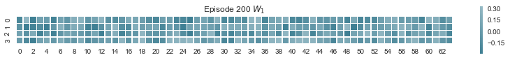
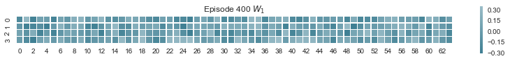
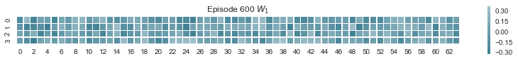
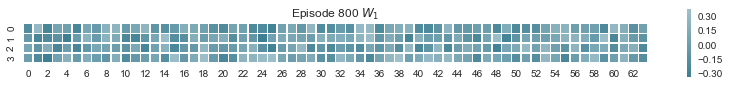
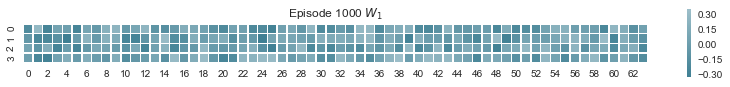
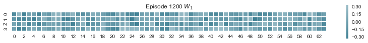
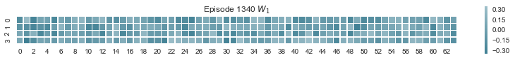
def plot_weights(weights, figsize=(7,5)):
    '''Heat map of weights to see which neurons play which role'''
    sns.set(style="white")
    f, ax = plt.subplots(len(weights), figsize=figsize)
    cmap = sns.diverging_palette(220, 10, as_cmap=True)

    for i, data in enumerate(weights):
        axi = ax if len(weights)==1 else ax[i]
        if isinstance(data, tuple):
            w, title = data
            axi.set_title(title)
        else:
            w = data

        sns.heatmap(w.asarray(), cmap=cmap, square=True, center=True, #annot=True,
                    linewidths=.5, cbar_kws={"shrink": .25}, ax=axi)

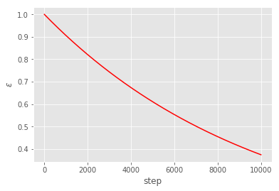
Exploration - exploitation trade-off

Note that the initial $\epsilon$ is set to 1 which implies we are entirely exploring but as steps increase we reduce exploration and start leveraging the learnt space to collect rewards (a.k.a. exploitation) as well.

def epsilon(steps):
    return MIN_EPSILON + (MAX_EPSILON - MIN_EPSILON) * np.exp(-LAMBDA * steps)
plt.plot(range(10000), [epsilon(x) for x in range(10000)], 'r')
plt.xlabel('step');plt.ylabel('$\epsilon$')

Text(0,0.5,'$\\epsilon$')

We are now ready to train our agent using DQN. Note this would take anywhere between 2-10 min and we stop whenever the learner hits the average reward of 200 over past 50 batches. One would get better results if they could train the learner until say one hits a reward of 200 or higher for say larger number of runs. This is left as an exercise.

TOTAL_EPISODES = 2000 if isFast else 3000

def run(agent):
    s = env.reset()
    R = 0

    while True:
        # Uncomment the line below to visualize the cartpole
        # env.render()

        # CNTK: explicitly setting to float32
        a = agent.act(s.astype(np.float32))

        s_, r, done, info = env.step(a)

        if done: # terminal state
            s_ = None

        agent.observe((s, a, r, s_))
        agent.replay()

        s = s_
        R += r

        if done:
            return R

agent = Agent()

episode_number = 0
reward_sum = 0
while episode_number < TOTAL_EPISODES:
    reward_sum += run(agent)
    episode_number += 1
    if episode_number % BATCH_SIZE_BASELINE == 0:
        print('Episode: %d, Average reward for episode %f.' % (episode_number,
                                                               reward_sum / BATCH_SIZE_BASELINE))
        if episode_number%200==0:
            plot_weights([(agent.brain.params['W1'], 'Episode %i $W_1$'%episode_number)], figsize=(14,5))
        if reward_sum / BATCH_SIZE_BASELINE > REWARD_TARGET:
            print('Task solved in %d episodes' % episode_number)
            plot_weights([(agent.brain.params['W1'], 'Episode %i $W_1$'%episode_number)], figsize=(14,5))
            break
        reward_sum = 0
agent.brain.model.save('dqn.mod')

Episode: 20, Average reward for episode 21.400000.
Episode: 40, Average reward for episode 24.450000.
Episode: 60, Average reward for episode 20.250000.
Episode: 80, Average reward for episode 20.900000.
Episode: 100, Average reward for episode 21.750000.
Episode: 120, Average reward for episode 16.400000.
Episode: 140, Average reward for episode 21.300000.
Episode: 160, Average reward for episode 20.150000.
Episode: 180, Average reward for episode 18.250000.
Episode: 200, Average reward for episode 16.250000.
Episode: 220, Average reward for episode 16.200000.
Episode: 240, Average reward for episode 14.000000.
Episode: 260, Average reward for episode 14.150000.
Episode: 280, Average reward for episode 16.000000.
Episode: 300, Average reward for episode 13.800000.
Episode: 320, Average reward for episode 13.650000.
Episode: 340, Average reward for episode 12.400000.
Episode: 360, Average reward for episode 12.900000.
Episode: 380, Average reward for episode 13.000000.
Episode: 400, Average reward for episode 11.550000.
Episode: 420, Average reward for episode 11.400000.
Episode: 440, Average reward for episode 12.400000.
Episode: 460, Average reward for episode 12.250000.
Episode: 480, Average reward for episode 11.650000.
Episode: 500, Average reward for episode 11.700000.
Episode: 520, Average reward for episode 12.100000.
Episode: 540, Average reward for episode 12.650000.
Episode: 560, Average reward for episode 11.300000.
Episode: 580, Average reward for episode 11.250000.
Episode: 600, Average reward for episode 11.000000.
Episode: 620, Average reward for episode 11.450000.
Episode: 640, Average reward for episode 10.850000.
Episode: 660, Average reward for episode 11.850000.
Episode: 680, Average reward for episode 12.200000.
Episode: 700, Average reward for episode 10.900000.
Episode: 720, Average reward for episode 11.700000.
Episode: 740, Average reward for episode 11.050000.
Episode: 760, Average reward for episode 11.400000.
Episode: 780, Average reward for episode 11.650000.
Episode: 800, Average reward for episode 11.200000.
Episode: 820, Average reward for episode 11.150000.
Episode: 840, Average reward for episode 11.900000.
Episode: 860, Average reward for episode 11.300000.
Episode: 880, Average reward for episode 11.300000.
Episode: 900, Average reward for episode 10.900000.
Episode: 920, Average reward for episode 11.050000.
Episode: 940, Average reward for episode 11.000000.
Episode: 960, Average reward for episode 11.350000.
Episode: 980, Average reward for episode 9.700000.
Episode: 1000, Average reward for episode 12.250000.
Episode: 1020, Average reward for episode 10.700000.
Episode: 1040, Average reward for episode 10.900000.
Episode: 1060, Average reward for episode 11.750000.
Episode: 1080, Average reward for episode 10.900000.
Episode: 1100, Average reward for episode 10.900000.
Episode: 1120, Average reward for episode 12.050000.
Episode: 1140, Average reward for episode 11.550000.
Episode: 1160, Average reward for episode 12.000000.
Episode: 1180, Average reward for episode 12.750000.
Episode: 1200, Average reward for episode 13.400000.
Episode: 1220, Average reward for episode 14.100000.
Episode: 1240, Average reward for episode 25.950000.
Episode: 1260, Average reward for episode 22.700000.
Episode: 1280, Average reward for episode 13.850000.
Episode: 1300, Average reward for episode 10.350000.
Episode: 1320, Average reward for episode 11.600000.
Episode: 1340, Average reward for episode 114.150000.
Task solved in 1340 episodes

If you run it, you should see something like

Episode: 20, Average reward for episode 20.700000.
Episode: 40, Average reward for episode 20.150000.
Episode: 60, Average reward for episode 21.100000.
...
Episode: 960, Average reward for episode 20.150000.
Episode: 980, Average reward for episode 26.700000.
Episode: 1000, Average reward for episode 32.900000.
Task solved in 1000 episodes

Task 1.1 Rewrite the model without using the layer lib.

Task 1.2 Play with different learners. Which one works better? Worse? Think about which parameters you would need to adapt when switching from one learner to the other.

Running the DQN model

env = gym.make('CartPole-v0')

num_episodes = 10  # number of episodes to run

modelPath = 'dqn.mod'
root = C.load_model(modelPath)

for i_episode in range(num_episodes):
    print(i_episode)
    observation = env.reset()  # reset environment for new episode
    done = False
    while not done:
        if not 'TEST_DEVICE' in os.environ:
            env.render()
        action = np.argmax(root.eval([observation.astype(np.float32)]))
        observation, reward, done, info  = env.step(action)

0
1
2
3
4
5
6
7
8
9

Part 2: Policy gradient (PG)

Goal:

$$\text{maximize } E [R | \pi_\theta]$$

Approach: 1. Collect experience (sample a bunch of trajectories through $(s,a)$ space) 2. Update the policy so that good experiences become more probable

Difference to DQN: * we don’t consider single $(s,a,r,s')$ transitions, but rather use whole episodes for the gradient updates * our parameters directly model the policy (output is an action probability), whereas in DQN they model the value function (output is raw score)

Rewards

Remember, we get +1 reward for every time step, in which we still were in the game.

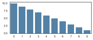
The problem: we normally do not know, which action led to a continuation of the game, and which was actually a bad one. Our simple heuristic: actions in the beginning of the episode are good, and those towards the end are likely bad (they led to losing the game after all).

def discount_rewards(r, gamma=0.999):
    """Take 1D float array of rewards and compute discounted reward """
    discounted_r = np.zeros_like(r)
    running_add = 0
    for t in reversed(range(0, r.size)):
        running_add = running_add * gamma + r[t]
        discounted_r[t] = running_add
    return discounted_r

discounted_epr = discount_rewards(np.ones(10))
f, ax = plt.subplots(1, figsize=(5,2))
sns.barplot(list(range(10)), discounted_epr, color="steelblue")

<matplotlib.axes._subplots.AxesSubplot at 0x2327a7ad128>

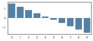
We normalize the rewards so that they tank below zero towards the end. gamma controls how late the rewards tank.

discounted_epr_cent = discounted_epr - np.mean(discounted_epr)
discounted_epr_norm = discounted_epr_cent/np.std(discounted_epr_cent)
f, ax = plt.subplots(1, figsize=(5,2))
sns.barplot(list(range(10)), discounted_epr_norm, color="steelblue")

<matplotlib.axes._subplots.AxesSubplot at 0x2327a4dfe48>

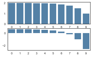
discounted_epr = discount_rewards(np.ones(10), gamma=0.5)
discounted_epr_cent = discounted_epr - np.mean(discounted_epr)
discounted_epr_norm = discounted_epr_cent/np.std(discounted_epr_cent)
f, ax = plt.subplots(2, figsize=(5,3))
sns.barplot(list(range(10)), discounted_epr, color="steelblue", ax=ax[0])
sns.barplot(list(range(10)), discounted_epr_norm, color="steelblue", ax=ax[1])

<matplotlib.axes._subplots.AxesSubplot at 0x23279db20f0>

Model: Policy Gradient

$$\begin{split}l_1 = relu( x W_1 + b_1) \\ l_2 = l_1 W_2 + b_2 \\ \pi(a|s) = sigmoid(l_2)\end{split}$$

Note: in policy gradient approach, the output of the dense layer is mapped into to a 0-1 range via the sigmoid function.

TOTAL_EPISODES = 2000 if isFast else 10000

D = 4  # input dimensionality
H = 10 # number of hidden layer neurons

observations = C.sequence.input_variable(STATE_COUNT, np.float32, name="obs")

W1 = C.parameter(shape=(STATE_COUNT, H), init=C.glorot_uniform(), name="W1")
b1 = C.parameter(shape=H, name="b1")
layer1 = C.relu(C.times(observations, W1) + b1)

W2 = C.parameter(shape=(H, ACTION_COUNT), init=C.glorot_uniform(), name="W2")
b2 = C.parameter(shape=ACTION_COUNT, name="b2")
score = C.times(layer1, W2) + b2
# Until here it was similar to DQN

probability = C.sigmoid(score, name="prob")

Running the PG model

Policy Search: The optimal policy search can be carried out with either gradient free approaches or by computing gradients over the policy space ($\pi_\theta$) which is parameterized by $\theta$. In this tutorial, we use the classic forward (loss.forward) and back (loss.backward) propagation of errors over the parameterized space $\theta$. In this case, $\theta = \{W_1, b_1, W_2, b_2\}$, our model parameters.

input_y = C.sequence.input_variable(1, np.float32, name="input_y")
advantages = C.sequence.input_variable(1, np.float32, name="advt")

loss = -C.reduce_mean(C.log(C.square(input_y - probability) + 1e-4) * advantages, axis=0, name='loss')

lr = 0.001
lr_schedule = C.learning_parameter_schedule_per_sample(lr)
sgd = C.sgd([W1, W2], lr_schedule)

gradBuffer = dict((var.name, np.zeros(shape=var.shape)) for var in loss.parameters if var.name in ['W1', 'W2', 'b1', 'b2'])

xs, hs, label, drs = [], [], [], []
running_reward = None
reward_sum = 0
episode_number = 1

observation = env.reset()

while episode_number <= TOTAL_EPISODES:
    x = np.reshape(observation, [1, STATE_COUNT]).astype(np.float32)

    # Run the policy network and get an action to take.
    prob = probability.eval(arguments={observations: x})[0][0][0]
    action = 1 if np.random.uniform() < prob else 0

    xs.append(x)  # observation
    # grad that encourages the action that was taken to be taken

    y = 1 if action == 0 else 0  # a "fake label"
    label.append(y)

    # step the environment and get new measurements
    observation, reward, done, info = env.step(action)
    reward_sum += float(reward)

    # Record reward (has to be done after we call step() to get reward for previous action)
    drs.append(float(reward))

    if done:
        # Stack together all inputs, hidden states, action gradients, and rewards for this episode
        epx = np.vstack(xs)
        epl = np.vstack(label).astype(np.float32)
        epr = np.vstack(drs).astype(np.float32)
        xs, label, drs = [], [], []  # reset array memory

        # Compute the discounted reward backwards through time.
        discounted_epr = discount_rewards(epr)
        # Size the rewards to be unit normal (helps control the gradient estimator variance)
        discounted_epr -= np.mean(discounted_epr)
        discounted_epr /= np.std(discounted_epr)

        # Forward pass
        arguments = {observations: epx, input_y: epl, advantages: discounted_epr}
        state, outputs_map = loss.forward(arguments, outputs=loss.outputs,
                                          keep_for_backward=loss.outputs)

        # Backward psas
        root_gradients = {v: np.ones_like(o) for v, o in outputs_map.items()}
        vargrads_map = loss.backward(state, root_gradients, variables=set([W1, W2]))

        for var, grad in vargrads_map.items():
            gradBuffer[var.name] += grad

        # Wait for some batches to finish to reduce noise
        if episode_number % BATCH_SIZE_BASELINE == 0:
            grads = {W1: gradBuffer['W1'].astype(np.float32),
                     W2: gradBuffer['W2'].astype(np.float32)}
            updated = sgd.update(grads, BATCH_SIZE_BASELINE)

            # reset the gradBuffer
            gradBuffer = dict((var.name, np.zeros(shape=var.shape))
                              for var in loss.parameters if var.name in ['W1', 'W2', 'b1', 'b2'])

            print('Episode: %d. Average reward for episode %f.' % (episode_number, reward_sum / BATCH_SIZE_BASELINE))

            if reward_sum / BATCH_SIZE_BASELINE > REWARD_TARGET:
                print('Task solved in: %d ' % episode_number)
                break

            reward_sum = 0

        observation = env.reset()  # reset env
        episode_number += 1
probability.save('pg.mod')

Episode: 20. Average reward for episode 24.550000.
Episode: 40. Average reward for episode 18.700000.
Episode: 60. Average reward for episode 20.750000.
Episode: 80. Average reward for episode 19.300000.
Episode: 100. Average reward for episode 19.750000.
Episode: 120. Average reward for episode 20.850000.
Episode: 140. Average reward for episode 20.150000.
Episode: 160. Average reward for episode 19.650000.
Episode: 180. Average reward for episode 15.150000.
Episode: 200. Average reward for episode 20.700000.
Episode: 220. Average reward for episode 18.500000.
Episode: 240. Average reward for episode 20.350000.
Episode: 260. Average reward for episode 17.700000.
Episode: 280. Average reward for episode 15.900000.
Episode: 300. Average reward for episode 21.700000.
Episode: 320. Average reward for episode 17.900000.
Episode: 340. Average reward for episode 17.850000.
Episode: 360. Average reward for episode 16.050000.
Episode: 380. Average reward for episode 19.450000.
Episode: 400. Average reward for episode 19.150000.
Episode: 420. Average reward for episode 18.950000.
Episode: 440. Average reward for episode 19.400000.
Episode: 460. Average reward for episode 21.550000.
Episode: 480. Average reward for episode 19.850000.
Episode: 500. Average reward for episode 17.500000.
Episode: 520. Average reward for episode 18.350000.
Episode: 540. Average reward for episode 23.050000.
Episode: 560. Average reward for episode 21.400000.
Episode: 580. Average reward for episode 25.350000.
Episode: 600. Average reward for episode 22.000000.
Episode: 620. Average reward for episode 22.700000.
Episode: 640. Average reward for episode 21.200000.
Episode: 660. Average reward for episode 24.050000.
Episode: 680. Average reward for episode 21.100000.
Episode: 700. Average reward for episode 22.500000.
Episode: 720. Average reward for episode 25.350000.
Episode: 740. Average reward for episode 24.400000.
Episode: 760. Average reward for episode 27.850000.
Episode: 780. Average reward for episode 27.200000.
Episode: 800. Average reward for episode 23.250000.
Episode: 820. Average reward for episode 26.350000.
Episode: 840. Average reward for episode 24.800000.
Episode: 860. Average reward for episode 26.350000.
Episode: 880. Average reward for episode 26.450000.
Episode: 900. Average reward for episode 21.750000.
Episode: 920. Average reward for episode 22.500000.
Episode: 940. Average reward for episode 26.350000.
Episode: 960. Average reward for episode 25.500000.
Episode: 980. Average reward for episode 32.050000.
Task solved in: 980

Solutions

observation = C.sequence.input_variable(STATE_COUNT, np.float32, name="s")

W1 = C.parameter(shape=(STATE_COUNT, H), init=C.glorot_uniform(), name="W1")
b1 = C.parameter(shape=H, name="b1")
layer1 = C.relu(C.times(observation, W1) + b1)

W2 = C.parameter(shape=(H, ACTION_COUNT), init=C.glorot_uniform(), name="W2")
b2 = C.parameter(shape=ACTION_COUNT, name="b2")
model = C.times(layer1, W2) + b2
W1.shape, b1.shape, W2.shape, b2.shape, model.shape

((4, 10), (10,), (10, 2), (2,), (2,))

# Correspoding layers implementation - Preferred solution
def create_model(input):
    with C.layers.default_options(init=C.glorot_uniform()):
        z = C.layers.Sequential([C.layers.Dense(H, name="layer1"),
                                 C.layers.Dense(ACTION_COUNT, name="layer2")])
        return z(input)

model = create_model(observation)

model.layer1.W.shape, model.layer1.b.shape, model.layer2.W.shape, model.layer2.b.shape, model.shape

((4, 10), (10,), (10, 2), (2,), (2,))