CNTK 205: Artistic Style Transfer
This tutorial shows how to transfer the style of one image to another. This allows us to take our ordinary photos and render them in the style of famous images or paintings.
Apart from creating nice looking pictures, in this tutorial you will learn how to load a pretrained VGG model into CNTK, how to get the gradient of a function with respect to an input variable (rather than a parameter), and how to use the gradient outside of CNTK.
We will follow the approach of Gatys et. al. with some of the improvements in Novak and Nikulin. While faster techniques exist, these are limited to transfering a particular style.
We begin by importing the necessary packages. In addition to the usual
suspects (numpy, scipy, and cntk) we will need PIL to
work with images, requests to download a pretrained model and
h5py to read in the weights of the pretrained model.
In [1]:
from __future__ import print_function
import numpy as np
from scipy import optimize as opt
import cntk as C
from PIL import Image
import requests
import h5py
import os
%matplotlib inline
import matplotlib.pyplot as plt

import cntk.tests.test_utils
cntk.tests.test_utils.set_device_from_pytest_env() # (only needed for our build system)
C.cntk_py.set_fixed_random_seed(1) # fix a random seed for CNTK components
The pretrained model is a VGG network which we originally got from this page. We host it in a place which permits easy downloading. Below we download it if it is not already available locally and load the weights into numpy arrays.
In [2]:
def download(url, filename):
    response = requests.get(url, stream=True)
    with open(filename, 'wb') as handle:
        for data in response.iter_content(chunk_size=2**20):
            if data: handle.write(data)


def load_vgg(path):
    f = h5py.File(path)
    layers = []
    for k in range(f.attrs['nb_layers']):
        g = f['layer_{}'.format(k)]
        n = g.attrs['nb_params']
        layers.append([g['param_{}'.format(p)][:] for p in range(n)])
    f.close()
    return layers

# Check for an environment variable defined in CNTK's test infrastructure
envvar = 'CNTK_EXTERNAL_TESTDATA_SOURCE_DIRECTORY'
def is_test(): return envvar in os.environ

path = 'vgg16_weights.bin'
url = 'https://cntk.ai/jup/models/vgg16_weights.bin'
# We check for the model locally
if not os.path.exists(path):
    # If not there we might be running in CNTK's test infrastructure
    if is_test():
        path = os.path.join(os.environ[envvar],'PreTrainedModels','Vgg16','v0',path)
    else:
        #If neither is true we download the file from the web
        print('downloading VGG model (~0.5GB)')
        download(url, path)
layers = load_vgg(path)
print('loaded VGG model')
loaded VGG model
Next we define the VGG network as a CNTK graph.
In [3]:
# A convolutional layer in the VGG network
def vggblock(x, arrays, layer_map, name):
    f = arrays[0]
    b = arrays[1]
    k = C.constant(value=f)
    t = C.constant(value=np.reshape(b, (-1, 1, 1)))
    y = C.relu(C.convolution(k, x, auto_padding=[False, True, True]) + t)
    layer_map[name] = y
    return y

# A pooling layer in the VGG network
def vggpool(x):
    return C.pooling(x, C.AVG_POOLING, (2, 2), (2, 2))


# Build the graph for the VGG network (excluding fully connected layers)
def model(x, layers):
    model_layers = {}
    def convolutional(z): return len(z) == 2 and len(z[0].shape) == 4
    conv = [layer for layer in layers if convolutional(layer)]
    cnt = 0
    num_convs = {1: 2, 2: 2, 3: 3, 4: 3, 5: 3}
    for outer in range(1,6):
        for inner in range(num_convs[outer]):
            x = vggblock(x, conv[cnt], model_layers, 'conv%d_%d' % (outer, 1+inner))
            cnt += 1
        x = vggpool(x)

    return x, C.combine([model_layers[k] for k in sorted(model_layers.keys())])
Defining the loss function
The interesting part in this line of work is the definition of a loss function that, when optimized, leads to a result that is close to both the content of one image, as well as the style of the other image. This loss contains multiple terms some of which are defined in terms of the VGG network we just created. Concretely, the loss takes a candidate image x and takes a weighted sum of three terms: the content loss, the style loss and the total variation loss:
where α and β are weights on the content loss and the style loss, respectively. We have normalized the weights so that the weight in front of the total variation loss is 1. How are each of these terms computed?
- The total variation loss T(x) is the simplest one to understand: It measures the average sum of squared differences among adjacent pixel values and encourages the result x to be a smooth image. We implement this by convolving the image with a kernel containing (-1,1) both horizontally and vertically, squaring the results and computing their average.
- The content loss is measuring the squared difference between the content image and x. We can measure this difference on the raw pixels or at various layers inside the VGG network. While we write the content loss as C(x) it implicitly depends on the content image we provide. However since that image is fixed we do not write this dependence explicitly.
- The style loss S(x) is similar to the content loss in that it also implicitly depends on another image. The main idea of Gatys et. al. was to define the style as the correlations among the activations of the network and measure the style loss as the squared difference between these correlations. In particular for a particular layer we compute a covariance matrix among the output channels averaging across all positions. The style loss is just the squared error between the covariance matrix induced by the style image and the covariance matrix induced by x. We are deliberately vague here as to which layer of the network in is used. Different implementations do this differently and below we will use a weighted sum of all the style losses of all layers.
Below we define these loss functions:
In [4]:
def flatten(x):
    assert len(x.shape) >= 3
    return C.reshape(x, (x.shape[-3], x.shape[-2] * x.shape[-1]))


def gram(x):
    features = C.minus(flatten(x), C.reduce_mean(x))
    return C.times_transpose(features, features)


def npgram(x):
    features = np.reshape(x, (-1, x.shape[-2]*x.shape[-1])) - np.mean(x)
    return features.dot(features.T)


def style_loss(a, b):
    channels, x, y = a.shape
    assert x == y
    A = gram(a)
    B = npgram(b)
    return C.squared_error(A, B)/(channels**2 * x**4)


def content_loss(a,b):
    channels, x, y = a.shape
    return C.squared_error(a, b)/(channels*x*y)


def total_variation_loss(x):
    xx = C.reshape(x, (1,)+x.shape)
    delta = np.array([-1, 1], dtype=np.float32)
    kh = C.constant(value=delta.reshape(1, 1, 1, 1, 2))
    kv = C.constant(value=delta.reshape(1, 1, 1, 2, 1))
    dh = C.convolution(kh, xx, auto_padding=[False])
    dv = C.convolution(kv, xx, auto_padding=[False])
    avg = 0.5 * (C.reduce_mean(C.square(dv)) + C.reduce_mean(C.square(dh)))
    return avg
Instantiating the loss
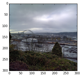
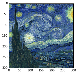
Now we are ready to instantiate a loss with two particular images. We
will use an image of Portland’s landscape and The Starry
Night by Vincent van
Gogh. We first define a few tuning parameters whose explanation is
below: - Depending on whether the code runs on a GPU or a CPU we resize
the images to 300 x 300 or 64 x 64 respectively and adjust the number of
iterations of optimization to speed up the process and for ease of
experimentation. You can use a larger size if you like the results. If
you only have a CPU you will have to wait a while. - The content weight
and style weight are the main parameters that affect the quality of the
resulting image. - The decay factor is a number in (0,1) which decides
how to weigh the contribution of each layer. Following Novak and
Nikulin, all layers contribute to
both the content loss and the style loss. The content loss weighs the
input more heavily and each later layer in the VGG network contributes
with a weight that is exponentially smaller with its distance from the
input. The style loss weighs the output of the VGG network more heavily
and each earlier layer in the VGG network contributes with a weight that
is exponentially smaller with its distance from the output. As in Novak
and Nikulin we use a decay factor of 0.5. - The inner and outer
parameters define how we are going to obtain our final result. We will
take outer snapshots during our search for the image that minimizes
the loss. Each snapshot will be taken after inner steps of
optimization. - Finally, a very important thing to know about our
pretrained network is how it was trained. In particular, a constant
vector was subtracted from all input images that contained the average
value for the red, green, and blue channels in the training set. This
makes the inputs zero centered which helps the training procedure. If we
do not subtract this vector our images will not look like the training
images and this will lead to bad results. This vector is referred to as
SHIFT below.
In [5]:
style_path = 'style.jpg'
content_path = 'content.jpg'

start_from_random = False
content_weight = 5.0
style_weight = 1.0
decay = 0.5

if is_test():
    outer = 2
    inner = 2
    SIZE = 64
else:
    outer = 10
    inner = 20
    SIZE = 300

SHIFT = np.reshape([103.939, 116.779, 123.68], (3, 1, 1)).astype('f')

def load_image(path):
    with Image.open(path) as pic:
        hw = pic.size[0] / 2
        hh = pic.size[1] / 2
        mh = min(hw,hh)
        cropped = pic.crop((hw - mh, hh - mh, hw + mh, hh + mh))
        array = np.array(cropped.resize((SIZE,SIZE), Image.BICUBIC), dtype=np.float32)
        return np.ascontiguousarray(np.transpose(array, (2,0,1)))-SHIFT

def save_image(img, path):
    sanitized_img = np.maximum(0, np.minimum(255, img+SHIFT))
    pic = Image.fromarray(np.uint8(np.transpose(sanitized_img, (1, 2, 0))))
    pic.save(path)

def ordered_outputs(f, binding):
    _, output_dict = f.forward(binding, f.outputs)
    return [np.squeeze(output_dict[out]) for out in f.outputs]

# download the images if they are not available locally
for local_path in content_path, style_path:
    if not os.path.exists(local_path):
        download('https://cntk.ai/jup/%s' % local_path, local_path)

# Load the images
style   = load_image(style_path)
content = load_image(content_path)

# Display the images
for img in content, style:
    plt.figure()
    plt.imshow(np.asarray(np.transpose(img+SHIFT, (1, 2, 0)), dtype=np.uint8))

# Push the images through the VGG network
# First define the input and the output
y = C.input_variable((3, SIZE, SIZE), needs_gradient=True)
z, intermediate_layers = model(y, layers)
# Now get the activations for the two images
content_activations = ordered_outputs(intermediate_layers, {y: [[content]]})
style_activations = ordered_outputs(intermediate_layers, {y: [[style]]})
style_output = np.squeeze(z.eval({y: [[style]]}))

# Finally define the loss
n = len(content_activations)
total = (1-decay**(n+1))/(1-decay) # makes sure that changing the decay does not affect the magnitude of content/style
loss = (1.0/total * content_weight * content_loss(y, content)
         + 1.0/total * style_weight * style_loss(z, style_output)
         + total_variation_loss(y))

for i in range(n):
    loss = (loss
        + decay**(i+1)/total * content_weight * content_loss(intermediate_layers.outputs[i], content_activations[i])
        + decay**(n-i)/total * style_weight   *   style_loss(intermediate_layers.outputs[i], style_activations[i]))
Optimizing the loss
Now we are finally ready to find the image that minimizes the loss we defined. We will use the optimization package in scipy and in particular the LBFGS method. LBFGS is a great optimization procedure which is very popular when computing the full gradient is feasible as is the case here.
Notice that we are computing the gradient with respect to the input. This is quite different from most other use cases where we compute the gradient with respect to the network parameters. By default, input variables do not ask for gradients, however we defined our input variable as
y = C.input_variable((3, SIZE, SIZE), needs_gradient=True)
which means that CNTK will compute the gradient with respect to this input variable as well.
The rest of the code is straightforward and most of the complexity comes from interacting with the scipy optimization package: - The optimizer works only with vectors of double precision so img2vec takes a (3,SIZE,SIZE) image and converts it to a vector of doubles - CNTK needs the input as an image but scipy is calling us back with a vector - CNTK computes a gradient as an image but scipy wants the gradient as a vector
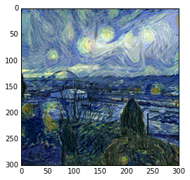
Besides these complexities we just start from the content image (or a random image), perform our optimization and display the final result.
In [6]:
# utility to convert a vector to an image
def vec2img(x):
    d = np.round(np.sqrt(x.size / 3)).astype('i')
    return np.reshape(x.astype(np.float32), (3, d, d))

# utility to convert an image to a vector
def img2vec(img):
    return img.flatten().astype(np.float64)

# utility to compute the value and the gradient of f at a particular place defined by binding
def value_and_grads(f, binding):
    if len(f.outputs) != 1:
        raise ValueError('function must return a single tensor')
    df, valdict = f.forward(binding, [f.output], set([f.output]))
    value = list(valdict.values())[0]
    grads = f.backward(df, {f.output: np.ones_like(value)}, set(binding.keys()))
    return value, grads

# an objective function that scipy will be happy with
def objfun(x, loss):
    y = vec2img(x)
    v, g = value_and_grads(loss, {loss.arguments[0]: [[y]]})
    v = np.reshape(v, (1,))
    g = img2vec(list(g.values())[0])
    return v, g

# the actual optimization procedure
def optimize(loss, x0, inner, outer):
    bounds = [(-np.min(SHIFT), 255-np.max(SHIFT))]*x0.size
    for i in range(outer):
        s = opt.minimize(objfun, img2vec(x0), args=(loss,), method='L-BFGS-B',
                         bounds=bounds, options={'maxiter': inner}, jac=True)
        print('objective : %s' % s.fun[0])
        x0 = vec2img(s.x)
        path = 'output_%d.jpg' % i
        save_image(x0, path)
    return x0

np.random.seed(98052)
if start_from_random:
    x0 = np.random.randn(3, SIZE, SIZE).astype(np.float32)
else:
    x0 = content
xstar = optimize(loss, x0, inner, outer)
plt.imshow(np.asarray(np.transpose(xstar+SHIFT, (1, 2, 0)), dtype=np.uint8))
objective : 52596.0
objective : 44182.2
objective : 42034.1
objective : 41035.2
objective : 40551.4
objective : 40256.1
objective : 40060.5
objective : 39937.1
objective : 39835.0
objective : 39754.1
Out[6]:
<matplotlib.image.AxesImage at 0x2825170d6a0>
In [7]:
# For testing purposes
objfun(xstar, loss)[0][0]
Out[7]:
39754.125