In [1]:
from IPython.display import Image
CNTK 105: Basic autoencoder (AE) with MNIST data
Prerequisites: We assume that you have successfully downloaded the MNIST data by completing the tutorial titled CNTK_103A_MNIST_DataLoader.ipynb.
Introduction
In this tutorial we introduce you to the basics of Autoencoders. An autoencoder is an artificial neural network used for unsupervised learning of efficient encodings. In other words, they are used for lossy data-specific compression that is learnt automatically instead of relying on human engineered features. The aim of an autoencoder is to learn a representation (encoding) for a set of data, typically for the purpose of dimensionality reduction.
The autoencoders are very specific to the data-set on hand and are different from standard codecs such as JPEG, MPEG standard based encodings. Once the information is encoded and decoded back to original dimensions some amount of information is lost in the process. Given these encodings are specific to data, autoencoders are not used for compression. However, there are two areas where autoencoders have been found very effective: denoising and dimensionality reduction.
Autoencoders have attracted attention since they have long been thought to be a potential approach for unsupervised learning. Truly unsupervised approaches involve learning useful representations without the need for labels. Autoencoders fall under self-supervised learning, a specific instance of supervised learning where the targets are generated from the input data.
Goal
Our goal is to train an autoencoder that compresses MNIST digits image to a vector of smaller dimension and then restores the image. The MNIST data comprises of hand-written digits with little background noise.
In [2]:
# Figure 1
Image(url="http://cntk.ai/jup/MNIST-image.jpg", width=300, height=300)
Out[2]:
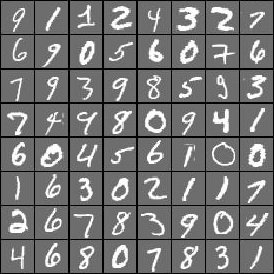
In this tutorial, we will use the MNIST hand-written digits data to show how images can be encoded and decoded (restored) using feed-forward networks. We will visualize the original and the restored images. We illustrate feed forward network based on two autoencoders: simple and deep autoencoder. More advanced autoencoders will be covered in future 200 series tutorials.
In [3]:
# Import the relevant modules
from __future__ import print_function # Use a function definition from future version (say 3.x from 2.7 interpreter)
import matplotlib.pyplot as plt
import numpy as np
import os
import sys

# Import CNTK
import cntk as C
import cntk.tests.test_utils
cntk.tests.test_utils.set_device_from_pytest_env() # (only needed for our build system)
C.cntk_py.set_fixed_random_seed(1) # fix a random seed for CNTK components

%matplotlib inline
There are two run modes: - Fast mode: isFast is set to True.
This is the default mode for the notebooks, which means we train for
fewer iterations or train / test on limited data. This ensures
functional correctness of the notebook though the models produced are
far from what a completed training would produce.
- Slow mode: We recommend the user to set this flag to
Falseonce the user has gained familiarity with the notebook content and wants to gain insight from running the notebooks for a longer period with different parameters for training.
In [4]:
isFast = True
Data reading
In this section, we will read the data generated in CNTK 103 Part A.
The data is in the following format:
|labels 0 0 0 0 0 0 0 1 0 0 |features 0 0 0 0 ...
                                              (784 integers each representing a pixel)
In this tutorial we are going to use the image pixels corresponding the
integer stream named “features”. We define a create_reader function
to read the training and test data using the CTF
deserializer.
The labels are 1-hot
encoded. We ignore them in
this tutorial.
We also check if the training and test data file has been downloaded and
available for reading by the create_reader function. In this
tutorial we are using the MNIST data you have downloaded using
CNTK_103A_MNIST_DataLoader notebook. The dataset has 60,000 training
images and 10,000 test images with each image being 28 x 28 pixels.
In [5]:
# Read a CTF formatted text (as mentioned above) using the CTF deserializer from a file
def create_reader(path, is_training, input_dim, num_label_classes):
    return C.io.MinibatchSource(C.io.CTFDeserializer(path, C.io.StreamDefs(
        labels_viz = C.io.StreamDef(field='labels', shape=num_label_classes, is_sparse=False),
        features   = C.io.StreamDef(field='features', shape=input_dim, is_sparse=False)
    )), randomize = is_training, max_sweeps = C.io.INFINITELY_REPEAT if is_training else 1)
In [6]:
# Ensure the training and test data is generated and available for this tutorial.
# We search in two locations in the toolkit for the cached MNIST data set.
data_found = False
for data_dir in [os.path.join("..", "Examples", "Image", "DataSets", "MNIST"),
                 os.path.join("data", "MNIST")]:
    train_file = os.path.join(data_dir, "Train-28x28_cntk_text.txt")
    test_file = os.path.join(data_dir, "Test-28x28_cntk_text.txt")
    if os.path.isfile(train_file) and os.path.isfile(test_file):
        data_found = True
        break

if not data_found:
    raise ValueError("Please generate the data by completing CNTK 103 Part A")
print("Data directory is {0}".format(data_dir))
Data directory is ..\Examples\Image\DataSets\MNIST
Model Creation (Simple AE)
We start with a simple single fully-connected feedforward network as encoder and as decoder (as shown in the figure below):
In [7]:
# Figure 2
Image(url="http://cntk.ai/jup/SimpleAEfig.jpg", width=200, height=200)
Out[7]:
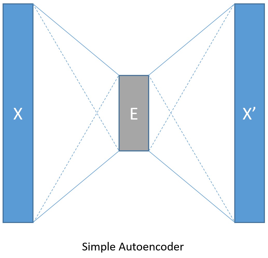
The input data is a set of hand written digits images each of 28 x 28
pixels. In this tutorial, we will consider each image as a linear array
of 784 pixel values. These pixels are considered as an input having 784
dimensions, one per pixel. Since the goal of the autoencoder is to
compress the data and reconstruct the original image, the output
dimension is same as the input dimension. We will compress the input to
mere 32 dimensions (referred to as the encoding_dim). Additionally,
since the maximum input value is 255, we normalize the input between 0
and 1.
In [8]:
input_dim = 784
encoding_dim = 32
output_dim = input_dim

def create_model(features):
    with C.layers.default_options(init = C.glorot_uniform()):
        # We scale the input pixels to 0-1 range
        encode = C.layers.Dense(encoding_dim, activation = C.relu)(features/255.0)
        decode = C.layers.Dense(input_dim, activation = C.sigmoid)(encode)

    return decode
Train and test the model
In previous tutorials, we have defined each of the training and testing phases separately. In this tutorial, we combine the two components in one place such that this template could be used as a recipe for your usage.
The train_and_test function performs two major tasks: - Train the
model - Evaluate the accuracy of the model on test data
For training:
The function takes a reader (
reader_train), a model function (model_func) and the target (a.k.alabel) as input. In this tutorial, we show how to create and pass your own loss function. We normalize thelabelfunction to emit value between 0 and 1 for us to compute the label error usingC.classification_errorfunction.We use Adam optimizer in this tutorial from a range of learners (optimizers) available in the toolkit.
For testing:
The function additionally takes a reader (reader_test) and evaluates the predicted pixel values made by the model against reference data, in this case the original pixel values for each image.
In [9]:
def train_and_test(reader_train, reader_test, model_func):

    ###############################################
    # Training the model
    ###############################################

    # Instantiate the input and the label variables
    input = C.input_variable(input_dim)
    label = C.input_variable(input_dim)

    # Create the model function
    model = model_func(input)

    # The labels for this network is same as the input MNIST image.
    # Note: Inside the model we are scaling the input to 0-1 range
    # Hence we rescale the label to the same range
    # We show how one can use their custom loss function
    # loss = -(y* log(p)+ (1-y) * log(1-p)) where p = model output and y = target
    # We have normalized the input between 0-1. Hence we scale the target to same range

    target = label/255.0
    loss = -(target * C.log(model) + (1 - target) * C.log(1 - model))
    label_error  = C.classification_error(model, target)

    # training config
    epoch_size = 30000        # 30000 samples is half the dataset size
    minibatch_size = 64
    num_sweeps_to_train_with = 5 if isFast else 100
    num_samples_per_sweep = 60000
    num_minibatches_to_train = (num_samples_per_sweep * num_sweeps_to_train_with) // minibatch_size


    # Instantiate the trainer object to drive the model training
    lr_per_sample = [0.00003]
    lr_schedule = C.learning_parameter_schedule_per_sample(lr_per_sample, epoch_size)

    # Momentum which is applied on every minibatch_size = 64 samples
    momentum_schedule = C.momentum_schedule(0.9126265014311797, minibatch_size)

    # We use a variant of the Adam optimizer which is known to work well on this dataset
    # Feel free to try other optimizers from
    # https://www.cntk.ai/pythondocs/cntk.learner.html#module-cntk.learner
    learner = C.fsadagrad(model.parameters,
                         lr=lr_schedule, momentum=momentum_schedule)

    # Instantiate the trainer
    progress_printer = C.logging.ProgressPrinter(0)
    trainer = C.Trainer(model, (loss, label_error), learner, progress_printer)

    # Map the data streams to the input and labels.
    # Note: for autoencoders input == label
    input_map = {
        input  : reader_train.streams.features,
        label  : reader_train.streams.features
    }

    aggregate_metric = 0
    for i in range(num_minibatches_to_train):
        # Read a mini batch from the training data file
        data = reader_train.next_minibatch(minibatch_size, input_map = input_map)

        # Run the trainer on and perform model training
        trainer.train_minibatch(data)
        samples = trainer.previous_minibatch_sample_count
        aggregate_metric += trainer.previous_minibatch_evaluation_average * samples

    train_error = (aggregate_metric*100.0) / (trainer.total_number_of_samples_seen)
    print("Average training error: {0:0.2f}%".format(train_error))

    #############################################################################
    # Testing the model
    # Note: we use a test file reader to read data different from a training data
    #############################################################################

    # Test data for trained model
    test_minibatch_size = 32
    num_samples = 10000
    num_minibatches_to_test = num_samples / test_minibatch_size
    test_result = 0.0

    # Test error metric calculation
    metric_numer    = 0
    metric_denom    = 0

    test_input_map = {
        input  : reader_test.streams.features,
        label  : reader_test.streams.features
    }

    for i in range(0, int(num_minibatches_to_test)):

        # We are loading test data in batches specified by test_minibatch_size
        # Each data point in the minibatch is a MNIST digit image of 784 dimensions
        # with one pixel per dimension that we will encode / decode with the
        # trained model.
        data = reader_test.next_minibatch(test_minibatch_size,
                                       input_map = test_input_map)

        # Specify the mapping of input variables in the model to actual
        # minibatch data to be tested with
        eval_error = trainer.test_minibatch(data)

        # minibatch data to be trained with
        metric_numer += np.abs(eval_error * test_minibatch_size)
        metric_denom += test_minibatch_size

    # Average of evaluation errors of all test minibatches
    test_error = (metric_numer*100.0) / (metric_denom)
    print("Average test error: {0:0.2f}%".format(test_error))

    return model, train_error, test_error
Let us train the simple autoencoder. We create a training and a test reader
In [10]:
num_label_classes = 10
reader_train = create_reader(train_file, True, input_dim, num_label_classes)
reader_test = create_reader(test_file, False, input_dim, num_label_classes)
model, simple_ae_train_error, simple_ae_test_error = train_and_test(reader_train,
                                                                    reader_test,
                                                                    model_func = create_model )
f:\projects\cntk\CNTK\bindings\python\cntk\learners\__init__.py:340: RuntimeWarning: When providing the schedule as a number, epoch_size is ignored
  warnings.warn('When providing the schedule as a number, epoch_size is ignored', RuntimeWarning)
 average      since    average      since      examples
    loss       last     metric       last
 ------------------------------------------------------
Learning rate per 1 samples: 3e-05
      544        544      0.846      0.846            64
      544        544      0.848       0.85           192
      544        543      0.868      0.883           448
      542        541      0.859      0.852           960
      538        533      0.848      0.837          1984
      496        456      0.754      0.662          4032
      385        275      0.584      0.417          8128
      303        221      0.442      0.301         16320
      250        197      0.339      0.236         32704
      208        167      0.257      0.176         65472
      173        138      0.182      0.108        131008
      142        111      0.116     0.0496        262080
Average training error: 10.57%
Average test error: 2.98%
Visualize simple AE results
In [11]:
# Read some data to run the eval
num_label_classes = 10
reader_eval = create_reader(test_file, False, input_dim, num_label_classes)

eval_minibatch_size = 50
eval_input_map = { input  : reader_eval.streams.features }

eval_data = reader_eval.next_minibatch(eval_minibatch_size,
                                  input_map = eval_input_map)

img_data = eval_data[input].asarray()

# Select a random image
np.random.seed(0)
idx = np.random.choice(eval_minibatch_size)

orig_image = img_data[idx,:,:]
decoded_image = model.eval(orig_image)[0]*255

# Print image statistics
def print_image_stats(img, text):
    print(text)
    print("Max: {0:.2f}, Median: {1:.2f}, Mean: {2:.2f}, Min: {3:.2f}".format(np.max(img),
                                                                              np.median(img),
                                                                              np.mean(img),
                                                                              np.min(img)))

# Print original image
print_image_stats(orig_image, "Original image statistics:")

# Print decoded image
print_image_stats(decoded_image, "Decoded image statistics:")
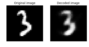
Original image statistics:
Max: 255.00, Median: 0.00, Mean: 24.07, Min: 0.00
Decoded image statistics:
Max: 252.06, Median: 0.44, Mean: 26.61, Min: 0.00
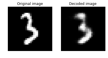
Let us plot the original and the decoded image. They should look visually similar.
In [12]:
# Define a helper function to plot a pair of images
def plot_image_pair(img1, text1, img2, text2):
    fig, axes = plt.subplots(nrows=1, ncols=2, figsize=(6, 6))

    axes[0].imshow(img1, cmap="gray")
    axes[0].set_title(text1)
    axes[0].axis("off")

    axes[1].imshow(img2, cmap="gray")
    axes[1].set_title(text2)
    axes[1].axis("off")
In [13]:
# Plot the original and the decoded image
img1 = orig_image.reshape(28,28)
text1 = 'Original image'

img2 = decoded_image.reshape(28,28)
text2 = 'Decoded image'

plot_image_pair(img1, text1, img2, text2)
Model Creation (Deep AE)
We do not have to limit ourselves to a single layer as encoder or decoder, we could instead use a stack of dense layers. Let us create a deep autoencoder.
In [14]:
# Figure 3
Image(url="http://cntk.ai/jup/DeepAEfig.jpg", width=500, height=300)
Out[14]:
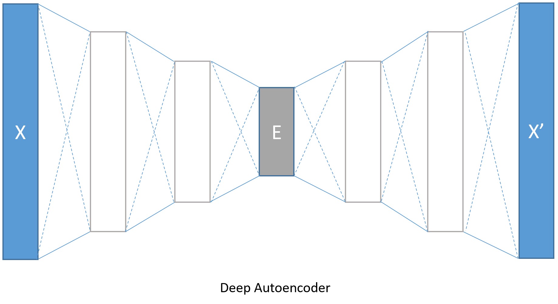
The encoding dimensions are 128, 64 and 32 while the decoding dimensions
are symmetrically opposite 64, 128 and 784. This increases the number of
parameters used to model the transformation and achieves lower error
rates at the cost of longer training duration and memory footprint. If
we train this deep encoder for larger number iterations by turning the
isFast flag to be False, we get a lower error and the
reconstructed images are also marginally better.
In [15]:
input_dim = 784
encoding_dims = [128,64,32]
decoding_dims = [64,128]

encoded_model = None

def create_deep_model(features):
    with C.layers.default_options(init = C.layers.glorot_uniform()):
        encode = C.element_times(C.constant(1.0/255.0), features)

        for encoding_dim in encoding_dims:
            encode = C.layers.Dense(encoding_dim, activation = C.relu)(encode)

        global encoded_model
        encoded_model= encode

        decode = encode
        for decoding_dim in decoding_dims:
            decode = C.layers.Dense(decoding_dim, activation = C.relu)(decode)

        decode = C.layers.Dense(input_dim, activation = C.sigmoid)(decode)
        return decode
In [16]:
num_label_classes = 10
reader_train = create_reader(train_file, True, input_dim, num_label_classes)
reader_test = create_reader(test_file, False, input_dim, num_label_classes)

model, deep_ae_train_error, deep_ae_test_error = train_and_test(reader_train,
                                                                reader_test,
                                                                model_func = create_deep_model)
f:\projects\cntk\CNTK\bindings\python\cntk\learners\__init__.py:340: RuntimeWarning: When providing the schedule as a number, epoch_size is ignored
  warnings.warn('When providing the schedule as a number, epoch_size is ignored', RuntimeWarning)
 average      since    average      since      examples
    loss       last     metric       last
 ------------------------------------------------------
Learning rate per 1 samples: 3e-05
      544        544      0.739      0.739            64
      544        544      0.794      0.822           192
      544        543      0.801      0.805           448
      543        542      0.817      0.831           960
      530        518      0.876      0.931          1984
      415        304      0.743      0.615          4032
      315        216      0.594      0.448          8128
      259        204      0.493      0.392         16320
      215        172      0.366       0.24         32704
      177        138      0.254      0.141         65472
      145        113      0.165     0.0759        131008
      120       95.9      0.104     0.0431        262080
Average training error: 9.52%
Average test error: 2.87%
Visualize deep AE results
In [17]:
# Run the same image as the simple autoencoder through the deep encoder
orig_image = img_data[idx,:,:]
decoded_image = model.eval(orig_image)[0]*255

# Print image statistics
def print_image_stats(img, text):
    print(text)
    print("Max: {0:.2f}, Median: {1:.2f}, Mean: {2:.2f}, Min: {3:.2f}".format(np.max(img),
                                                                              np.median(img),
                                                                              np.mean(img),
                                                                              np.min(img)))

# Print original image
print_image_stats(orig_image, "Original image statistics:")

# Print decoded image
print_image_stats(decoded_image, "Decoded image statistics:")
Original image statistics:
Max: 255.00, Median: 0.00, Mean: 24.07, Min: 0.00
Decoded image statistics:
Max: 248.16, Median: 0.02, Mean: 22.87, Min: 0.00
Let us plot the original and the decoded image with the deep autoencoder. They should look visually similar.
In [18]:
# Plot the original and the decoded image
img1 = orig_image.reshape(28,28)
text1 = 'Original image'

img2 = decoded_image.reshape(28,28)
text2 = 'Decoded image'

plot_image_pair(img1, text1, img2, text2)
We have shown how to encode and decode an input. In this section we will explore how we can compare one to another and also show how to extract an encoded input for a given input. For visualizing high dimension data in 2D, t-SNE is probably one of the best methods. However, it typically requires relatively low-dimensional data. So a good strategy for visualizing similarity relationships in high-dimensional data is to encode data into a low-dimensional space (e.g. 32 dimensional) using an autoencoder first, extract the encoding of the input data followed by using t-SNE for mapping the compressed data to a 2D plane.
We will use the deep autoencoder outputs to: - Compare two images and - Show how we can retrieve an encoded (compressed) data.
First we need to read some image data along with their labels.
In [19]:
# Read some data to run get the image data and the corresponding labels
num_label_classes = 10
reader_viz = create_reader(test_file, False, input_dim, num_label_classes)

image = C.input_variable(input_dim)
image_label = C.input_variable(num_label_classes)

viz_minibatch_size = 50

viz_input_map = {
    image  : reader_viz.streams.features,
    image_label  : reader_viz.streams.labels_viz
}

viz_data = reader_eval.next_minibatch(viz_minibatch_size,
                                  input_map = viz_input_map)

img_data   = viz_data[image].asarray()
imglabel_raw = viz_data[image_label].asarray()
In [20]:
# Map the image labels into indices in minibatch array
img_labels = [np.argmax(imglabel_raw[i,:,:]) for i in range(0, imglabel_raw.shape[0])]

from collections import defaultdict
label_dict=defaultdict(list)
for img_idx, img_label, in enumerate(img_labels):
    label_dict[img_label].append(img_idx)

# Print indices corresponding to 3 digits
randIdx = [1, 3, 9]
for i in randIdx:
    print("{0}: {1}".format(i, label_dict[i]))
1: [7, 24, 39, 44, 46]
3: [1, 13, 18, 26, 37, 40, 43]
9: [8, 12, 23, 28, 42, 49]
We will compute cosine
distance between
two images using scipy.
In [21]:
from scipy import spatial

def image_pair_cosine_distance(img1, img2):
    if img1.size != img2.size:
        raise ValueError("Two images need to be of same dimension")
    return 1 - spatial.distance.cosine(img1, img2)
In [22]:
# Let s compute the distance between two images of the same number
digit_of_interest = 6

digit_index_list = label_dict[digit_of_interest]

if len(digit_index_list) < 2:
    print("Need at least two images to compare")
else:
    imgA = img_data[digit_index_list[0],:,:][0]
    imgB = img_data[digit_index_list[1],:,:][0]

    # Print distance between original image
    imgA_B_dist = image_pair_cosine_distance(imgA, imgB)
    print("Distance between two original image: {0:.3f}".format(imgA_B_dist))

    # Plot the two images
    img1 = imgA.reshape(28,28)
    text1 = 'Original image 1'

    img2 = imgB.reshape(28,28)
    text2 = 'Original image 2'

    plot_image_pair(img1, text1, img2, text2)

    # Decode the encoded stream
    imgA_decoded =  model.eval([imgA])[0]
    imgB_decoded =  model.eval([imgB])   [0]
    imgA_B_decoded_dist = image_pair_cosine_distance(imgA_decoded, imgB_decoded)

    # Print distance between original image
    print("Distance between two decoded image: {0:.3f}".format(imgA_B_decoded_dist))

    # Plot the two images
    # Plot the original and the decoded image
    img1 = imgA_decoded.reshape(28,28)
    text1 = 'Decoded image 1'

    img2 = imgB_decoded.reshape(28,28)
    text2 = 'Decoded image 2'

    plot_image_pair(img1, text1, img2, text2)
Distance between two original image: 0.294
Distance between two decoded image: 0.351
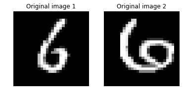
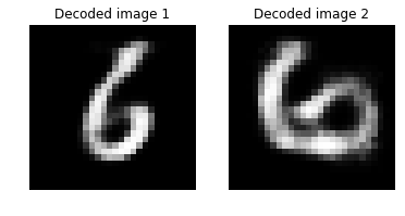
Note: The cosine distance between the original images comparable to the distance between the corresponding decoded images. A value of 1 indicates high similarity between the images and 0 indicates no similarity.
Let us now see how to get the encoded vector corresponding to an input
image. This should have the dimension of the choke point in the network
shown in the figure with the box labeled E.
In [23]:
imgA = img_data[digit_index_list[0],:,:][0]
imgA_encoded =  encoded_model.eval([imgA])

print("Length of the original image is {0:3d} and the encoded image is {1:3d}".format(len(imgA),
                                                                                      len(imgA_encoded[0])))
print("\nThe encoded image: ")
print(imgA_encoded[0])
Length of the original image is 784 and the encoded image is  32

The encoded image:
[ 14.24417496  11.13341045  11.24246407   4.64616632   0.           6.89158678
  23.79421425  18.19504166  17.70633888   0.           0.          28.18136215
  13.94447613  17.40437126  16.58884048   7.5404644   14.78264236
  20.94945335   5.16527224  19.49497986  12.03796673  19.87505722
  13.01367664   8.0799036    6.24639368   0.          14.11477566
  20.0975914    4.01841021  10.9685421   16.97727776  13.98702526]
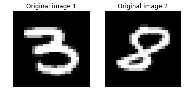
Let us compare the distance between different digits.
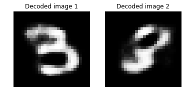
In [24]:
digitA = 3
digitB = 8

digitA_index = label_dict[digitA]
digitB_index = label_dict[digitB]

imgA = img_data[digitA_index[0],:,:][0]
imgB = img_data[digitB_index[0],:,:][0]

# Print distance between original image
imgA_B_dist = image_pair_cosine_distance(imgA, imgB)
print("Distance between two original image: {0:.3f}".format(imgA_B_dist))

# Plot the two images
img1 = imgA.reshape(28,28)
text1 = 'Original image 1'

img2 = imgB.reshape(28,28)
text2 = 'Original image 2'

plot_image_pair(img1, text1, img2, text2)

# Decode the encoded stream
imgA_decoded =  model.eval([imgA])[0]
imgB_decoded =  model.eval([imgB])[0]
imgA_B_decoded_dist = image_pair_cosine_distance(imgA_decoded, imgB_decoded)

#Print distance between original image
print("Distance between two decoded image: {0:.3f}".format(imgA_B_decoded_dist))

# Plot the original and the decoded image
img1 = imgA_decoded.reshape(28,28)
text1 = 'Decoded image 1'

img2 = imgB_decoded.reshape(28,28)
text2 = 'Decoded image 2'

plot_image_pair(img1, text1, img2, text2)
Distance between two original image: 0.376
Distance between two decoded image: 0.424
Print the results of the deep encoder test error for regression testing
In [25]:
# Simple autoencoder test error
print(simple_ae_test_error)
2.97620738737
In [26]:
# Deep autoencoder test error
print(deep_ae_test_error)
2.87243351221
Suggested tasks
- Try different activation functions.
- Find which images are more similar to one another (a) using original image and (b) decoded image.
- Try using mean square error as the loss function. Does it improve the performance of the encoder in terms of reduced errors.
- Can you try different network structure to reduce the error further. Explain your observations.
- Can you use a different distance metric to compute similarity between the MNIST images.
- Try a deep encoder with [1000, 500, 250, 128, 64, 32]. What is the training error for same number of iterations?